Introduction (TS 3.1, 3.3, 3.6, S6) #

Overview of main models #

We are now ready to introduce the main models with full generality, and to discuss an overall estimation, fitting, and forecasting approach. The main models we will review are:

• Autoregressive models of order \(p\), denoted \(\alert{AR(p)}\): $$x_t=\alpha+\phi_1x_{t-1}+\phi_2 x_{t-2}+\cdots+\phi_p x_{t-p}+w_t,$$ where \(\alpha=\mu(1-\phi_1-\phi_2-\cdots-\phi_p)\).
• Moving averages of order \(q\), denoted \(\alert{MA(q)}\): $$x_t=w_t+\theta_1w_{t-1}+\theta_2 w_{t-2}+\cdots+\theta_q w_{t-q}.$$
• \(\alert{ARMA(p,q)}\) models, which are a combination of the above: $$x_t=\phi_1x_{t-1}+\cdots+\phi_p x_{t-p}+w_t+\theta_1w_{t-1}+\cdots+\theta_q w_{t-q}$$

Variations #

• \(\alert{ARIMA(p,d,q)}\) models, which reduce to \(ARMA(p,q)\) when differenced \(d\) times.
• Multiplicative seasonal ARIMA models:
  • Pure seasonal autoregressive moving average \(\alert{ARMA(P,Q)_s}\) models
  • Multiplicative seasonal autoregressive moving average models
  • Seasonal autoregressive integrated moving average models
• Multivariate time series—Vector Auto-Regressive \(\alert{VAR(p)}\) models
• Extra models mentioned by the CS2 syllabus:
  • bilinear model
  • threshold autoregressive model
  • \(ARCH(p)\) models

Partial Autocorrelation Function (PACF) #

Motivation #

• There is one more property we need to introduce, the Partial Autocorrelation Function (PACF).
• The ACF can help identify \(q\) for a \(MA(q)\) model, because it should be 0 for lags \(>q\)
• However, the order of an \(AR(p)\) or \(ARMA(p,q)\) model cannot be recognised from the ACF.
• What we need for autoregressive models is a measure of dependence at two different points in time,
  with the effect of the other points in time removed.
• We will remove the linear effect of all variables in-between, and so by increasing the lag iteratively, this partial correlation should be 0 after some lag ( \(p\) for \(AR(p)\))

Reminder: partial correlation #

• Let \(X\), \(Y\), and \(Z\) be random variables.
• The partial correlation between \(X\) and \(Y\), given \(Z\) is obtained by
  • Regressing \(X\) on \(Z\) to obtain \(\hat{X}\);
  • Regressing \(Y\) on \(Z\) to obtain \(\hat{Y}\),
• Then the partial correlation is $$\rho_{XY|Z}=\text{corr}\{X-\hat{X},Y-\hat{Y}\}.$$
• In the special case where the random variables are multivariate normal (and hence dependence is linear), $$\rho_{XY|Z}=\text{corr}\{X,Y|Z\}.$$ (Otherwise, \(\hat{X}\) and \(\hat{Y}\) are only linear projections, not the full story.)

The partial autocorrelation function (PACF) #

The partial autocorrelation function (PACF) of a stationary process, \(x_t\), denoted \(\phi_{hh}\), for \(h = 1, 2,\ldots\), is $$\phi_{11}=\text{corr}(x_{t+1},x_t)=\rho(1),$$ and $$\phi_{hh}=\text{corr}(x_{t+h}-\hat{x}_{t+h},x_t-\hat{x}_t),\quad h\ge 2. $$ Note:

• The PACF, \(\phi_{hh}\), is the correlation between \(x_{t+h}\) and \(x_t\) with the linear dependence of \(\{x_{t+1},\ldots, x_{t+h-1}\}\) on each, removed.
• The PACF of an \(AR(p)\) model will be 0 for \(h>p\).
• The R function pacf will display a sample \(\phi_{hh}\) for \(h>0\).

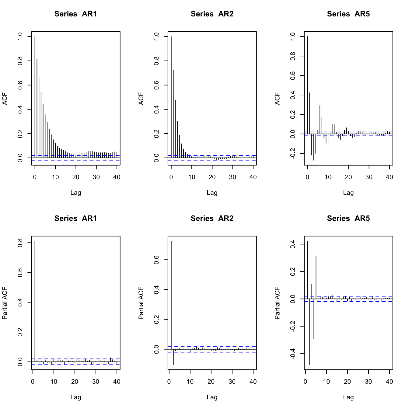
Examples of AR PACFs #

set.seed(2)
AR1 <- arima.sim(list(order = c(1, 0, 0), ar = 0.8), n = 10000)
AR2 <- arima.sim(list(order = c(2, 0, 0), ar = c(0.8, -0.1)),
  n = 10000)
AR5 <- arima.sim(list(order = c(5, 0, 0), ar = c(0.8, -0.8, 0.5,
  -0.5, 0.3)), n = 10000)
par(mfrow = c(2, 3))
acf(AR1)
acf(AR2)
acf(AR5)
pacf(AR1)
pacf(AR2)
pacf(AR5)

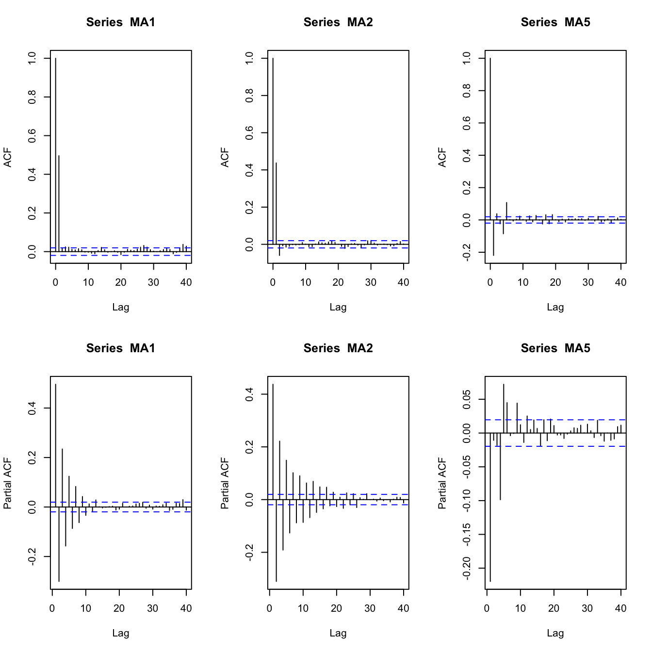
Examples of MA PACFs #

set.seed(2)
MA1 <- arima.sim(list(order = c(0, 0, 1), ma = 0.8), n = 10000)
MA2 <- arima.sim(list(order = c(0, 0, 2), ma = c(0.8, -0.1)),
  n = 10000)
MA5 <- arima.sim(list(order = c(0, 0, 5), ma = c(0.8, -0.8, 0.5,
  -0.5, 0.3)), n = 10000)
par(mfrow = c(2, 3))
acf(MA1)
acf(MA2)
acf(MA5)
pacf(MA1)
pacf(MA2)
pacf(MA5)

\(AR(p)\) models (TS 3.1, 3.3, 3.6, S6) #

Definition #

\(AR(p)\) models #

An autoregressive model of order \(p\) \(AR(p)\) is of the form $$x_t=\alpha+\phi_1x_{t-1}+\phi_2 x_{t-2}+\cdots+\phi_p x_{t-p}+w_t,$$ where \(x_t\) is stationary, \(w_t\sim \text{wn}(0,\sigma_w^2)\), \(\phi_1,\phi_2,\ldots,\phi_p\) are constants \((\phi_p\neq0)\), and where \(\alpha=\mu(1-\phi_1-\phi_2-\cdots-\phi_p)\).

Assume \(\alpha=0\) and rewrite $$(1-\phi_1B-\phi_2 B^2-\cdots-\phi_pB^p)x_t=w_t \quad\text{or}\quad \alert{\phi(B)x_t=w_t}.$$ Note:

• Unless stated otherwise we assume \(\alpha=0\). The mean of \(x_t\) is then zero.
• Recall that here the regressors \(x_{t-1},\ldots,x_{t-p}\) are random components (as opposed to the ‘usual’ regression).
• The autoregressive operator is defined as $$\phi(B)=(1-\phi_1B-\phi_2 B^2-\cdots-\phi_pB^p),$$ the roots of which will be crucial for the analysis.

Example: AR(1) model #

An \(AR(1)\) is $$\begin{array}{rcl} x_t&=&\phi x_{t-1}+w_t\\ &=&\phi(\phi x_{t-2}+w_{t-1})+w_t \\ &\vdots& \\ &=& \phi^k x_{t-k}+\sum_{j=0}^{k-1}\phi^j w_{t-j} \end{array}$$ If one continues to iterate backwards, one gets (provided \(|\phi|<1\) and \(\sup_t Var(x_t)<\infty\)) $$x_t = \sum_{j=0}^\infty \phi^j w_{t-j},$$ a linear process! This is called the stationary solution of the model.

The stationary solution of the model has mean $$E[x_t]=\sum_{j=0}^\infty \phi^j E[w_{t-j}] = 0,$$ and autocovariance function (see (3.7) in TS) $$\gamma(h) = \frac{\sigma_w^2 \phi^h}{1-\phi^2}, \quad h\ge 0.$$ (remember \(\gamma(h)=\gamma(-h)\)) The ACF of an \(AR(1)\) is $$\rho(h)=\frac{\gamma(h)}{\gamma(0)}=\phi^h, \quad h\ge0,$$ and \(\rho(h)\) satisfies the recursion $$\rho(h)=\phi \rho(h-1), \quad h=1,2,\ldots.$$

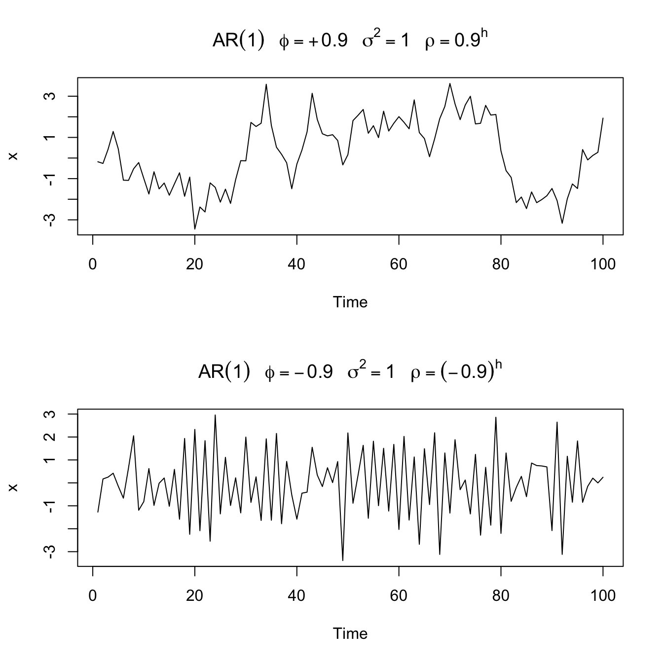
Sample paths of \(AR(1)\) processes #

par(mfrow = c(2, 1))
plot(arima.sim(list(order = c(1, 0, 0), ar = 0.9), n = 100),
  ylab = "x", main = (expression(AR(1) ~ ~~phi == +0.9 ~ ~~sigma^2 ==
    1 ~ ~~rho == 0.9^h)))
plot(arima.sim(list(order = c(1, 0, 0), ar = -0.9), n = 100),
  ylab = "x", main = (expression(AR(1) ~ ~~phi == -0.9 ~ ~~sigma^2 ==
    1 ~ ~~rho == (-0.9)^h)))

Stationarity (and Causality) #

Stationarity of \(AR(p)\) processes #

The time series process \(x_t\) is stationary and causal if, and only if, the roots of the characteristic polynomial $$1-\phi_1z-\phi_2 z^2 - \cdots -\phi_p z^p = \phi(z) = 0$$ (which can be complex numbers) are all greater than 1 in absolute value (outside the unit circle).

We will get a sense of why as we make our way through this module.

ACF and PACF #

Autocovariances #

Remember that for stationary \(x_t=\sum_{j=1}^p \phi_j x_{t-j}+w_t\) we have $$\gamma(k)=Cov\left(\sum_{j=1}^p \phi_j x_{t-j}+w_t,x_{t-k}\right) = \sum_{j=1}^p \phi_j \gamma(k-j)\quad\text{for }k\ge 0.$$ This is a \(p\)-th order difference equation with constant coefficients with solution (see TS 3.2) $$\gamma(k)=\sum_{j=1}^p A_j z_j^{-k}\text{ for all }k\ge 0,$$ where \(z_1, \ldots, z_p\) are the \(p\) roots of the characteristic polynomial \(\phi(z)=0\), and \(A_1, \ldots, A_p\) are constants depending on the initial values.

R can calculate this for you (code is provided later).

Note:

• we expect \(\gamma(k)\rightarrow 0\) as \(k\rightarrow \infty\) for stationary \(x_t\)
• this is equivalent to \(|z_j|>1\) for all \(j\)
• this is equivalent to our iff condition for \(x_t\) to be stationary and causal

Yule-Walker equations #

• We have a solution form for \(\gamma(k)\), but no explicit solution yet. These need to be solved for.
• Sometimes, it is quicker to use the so-called “Yule-Walker equations”. Consider the equation for an \(AR(p)\) model with \(\mu=0\), multiply by \(x_{t-k}\), take expectations to get $$\begin{array}{rcl} Cov(x_t,x_{t-k})&=&\phi_1 Cov(x_{t-1},x_{t-k}) + \phi_2 Cov(x_{t-2},x_{t-k}) + \ldots \\ && + \phi_p Cov(x_{t-p},x_{t-k})+Cov(w_t,x_{t-k}),\; 0\le k\le p, \end{array}$$ that is, $$\gamma(k)=\phi_1 \gamma(k-1)+\phi_2 \gamma(k-2)+\ldots+\phi_p \gamma(k-p)+\sigma^2_w 1_{\{k=0\}}, \; 0\le k\le p.$$ This is solvable thanks to the fact that \(\gamma(k)=\gamma(-k)\).
• A matrix representation will be introduced later

Example #

• For an \(AR(3)\) model we have $$\begin{array}{rcl} \gamma(3) &=& \phi_1 \gamma(2)+\phi_2\gamma(1)+\phi_3\gamma(0), \\ \gamma(2) &=& \phi_1 \gamma(1)+\phi_2\gamma(0)+\phi_3\gamma(1), \\ \gamma(1) &=& \phi_1 \gamma(0)+\phi_2\gamma(1)+\phi_3\gamma(2), \\ \gamma(0) &=& \phi_1 \gamma(1)+\phi_2\gamma(2)+\phi_3\gamma(3) +\sigma_w^2. \end{array}$$
• The second and third equations can be solved linearly to obtain expressions for \(\gamma(1)\) and \(\gamma(2)\) as a constant times \(\gamma(0)\), which yields explicitly \(\rho(1)\) and \(\rho(2)\). ( Remember \(\rho(k)=\gamma(k)/\gamma(0)\), \(\rho(0)=1\) ) $$\begin{array}{rcl} \rho(2) &=& \phi_1 \rho(1)+\phi_2+\phi_3\rho(1), \\ \rho(1) &=& \phi_1+ \phi_2\rho(1)+\phi_3\rho(2), +\sigma_w^2. \end{array}$$
• For numerical values of \(\gamma(1)\) and \(\gamma(2)\), and indeed the others, too, the system needs to be solved for.
  The matrix representation will help.

ACF #

As illustrated above $$\rho(h)=\sum_{j=1}^p \phi_j \rho(k-j),$$ because \(\rho(h)=\gamma(h)/\gamma(0).\)

Note:

• For stationary and causal AR, \(|z_i|>1\), \(i=1,\ldots,r\) ( \(r\le p\) distinct roots)
• If all the roots are real, then \(\rho(h)\) dampens exponentially fast to zero as \(h\rightarrow \infty\).
• If some of the roots are complex, then they will be in conjugate pairs and \(\rho(h)\) will dampen, in a sinusoidal fashion, exponentially fast to zero as \(h\rightarrow \infty\). In this case, the time series may appear to be cyclic in nature.
• This property flows on to ARMA models.

PACF #

When \(h>p\) the regression of \(x_{t+h}\) on \(\{x_{t+1},\ldots,x_{t+h-1}\}\) is $$\hat{x}_{t+h}=\sum_{j=1}^{\alert{p}} \phi_j x_{t+h-j},\quad \alert{h>p}.$$ This is not a typo, it is a really nice result! (see TS for a proof).

[why? because this means that \(\hat{x}_{t+h}=x_{t+h}-w_{t+h}\)]

This means that \(x_t-\hat{x}_t\), which will depend only on \(\{w_{t+h-1},w_{t+h-2},\ldots\}\), has no overlap with \(x_{t+h}-\hat{x}_{t+h}=w_{t+h}\)

Hence the PACF $$\phi_{hh}=\text{corr}(x_{t+h}-\hat{x}_{t+h},x_t-\hat{x}_t)=\text{corr}(w_{t+h},x_t-\hat{x}_t) =0, \quad h>p.$$

In summary, we know that $$\phi_{hh} = 0, \text{ for all }h>p$$ “by design” (we wanted a measure that would die down beyond \(p\) for diagnostic reasons).

“In-between”, we have that $$\phi_{11},\ldots,\phi_{pp}$$ are not necessarily 0.

Furthermore, it can be shown that $$\phi_{pp} =\phi_p,$$ a really nice feature.

Explosive AR models and causality #

Remember the random walk (an \(AR(1)\) with \(\phi=1\)) $$x_t=x_{t-1}+ w_t$$ is not stationary. This was because \(x_{t-1}\) includes all past \(w_t\)’s, leading to an exploding variance.

Examination of the \(AR(1)\) representation $$x_t = \sum_{j=0}^\infty \phi^j w_{t-j}$$ suggests that the key to contain explosion is with \(\phi\). If \(|\phi^j|\) increases without bound as \(j\rightarrow \infty\) the expected value of this quantity won’t converge. Explosive processes quickly become large in magnitude, leading to unstationarity.

Unfortunately not all AR models are stationary. For the random walk, \(\phi=1\) and it is not stationary. What are the values of \(\phi\) so that this does not happen?

Assume \(|\phi|>1\). Write (by iterating forward \(k\) steps) $$\begin{array}{rcl} x_{t}&=&\phi^{-1} x_{t+1}-\phi^{-1}w_{t+1} \\ &=&\phi^{-1}\left( \phi^{-1} x_{t+2}-\phi^{-1}w_{t+2}\right) -\phi^{-1}w_{t+1} \\ &\vdots& \\ &=& \phi^{-k}x_{t+k}-\sum_{j=1}^{k-1} \phi^{-j} w_{t+j} \end{array}$$

Because \(|\phi|^{-1} <1\), this result suggests the future dependent \(AR(1)\) model $$x_t=-\sum_{j=1}^{\infty} \phi^{-j} w_{t+j}.$$ This is of the \(AR(1)\) form \(x_t=\phi x_{t-1} + w_t\), but it is useless because it requires us to know the future to be able to predict the future!

When a process does not depend on the future— such as \(AR(1)\) when \(|\phi|<1\)— we will say the process is causal.

The model above with \(|\phi|>1\) is stationary, but it is also future dependent, and hence is not causal.

Here is the lesson for \(p>1\):

• stationary and causal are not equivalent conditions
• depending on the parameters of your \(AR(p)\) model, you may have a future dependent model without knowing it: when \(p>1\) it is not obvious by just looking at the parameters \(\phi_j\)
• that’s why the condition above stated “stationary and causal”
• this is further discussed in the ARMA section, where the argument above is further generalised to \(p>1\)

\(MA(q)\) models (TS 3.1, 3.3, 3.6, S6) #

Definition #

\(MA(q)\) models #

The moving average model of order \(q\) \(MA(q)\) is of the form $$x_t=w_t+\theta_1 w_{t-1}+\theta_2 w_{t-2}+\cdots+\theta_q w_{t-q}=\theta(B) w_t,$$ where \(w_t\sim \text{wn}(0,\sigma_w^2)\) and \(\theta_1, \theta_2, \ldots, \theta_q\) \((\theta_q\neq 0)\) are parameters.

Note:

• The AR combines linearly the \(x_t\)’s, whereas the MA combines linearly the \(w_t\)’s.
• The moving average operator is defined as $$\theta(B)=1+\theta_1 B+\theta_2 B^2+\cdots +\theta_q B^q.$$
• Unlike the AR, the MA is stationary for any value of the parameters \(\theta\)’s

Example: \(MA(1)\) model #

An \(MA(1)\) is $$x_t=w_t+\theta w_{t-1}.$$ Hence, $$E[x_t]=0,$$ and $$\gamma(h)=\left\{\begin{array}{lc} (1+\theta^2)\sigma_w^2 & h=0, \\ \theta \sigma_w^2 & h=1, \\ 0 & h>1, \end{array}\right.$$ and the ACF is $$\rho(h)=\left\{\begin{array}{lc} (1 & h=0) \\ \frac{\theta}{(1+\theta^2)} & h=1, \\ 0 & h>1. \end{array}\right.$$ Furthermore \(|\rho(1)| \le 1/2\) for all values of \(\theta\).

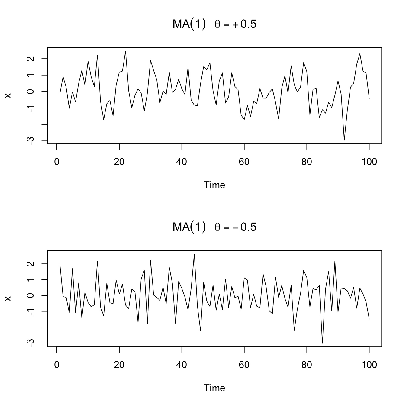
Sample paths of \(MA(1)\) processes #

par(mfrow = c(2, 1))
plot(arima.sim(list(order = c(0, 0, 1), ma = 0.5), n = 100),
  ylab = "x", main = (expression(MA(1) ~ ~~theta == +0.5)))
plot(arima.sim(list(order = c(0, 0, 1), ma = -0.5), n = 100),
  ylab = "x", main = (expression(MA(1) ~ ~~theta == -0.5)))

Non-uniqueness and invertibility #

• Note that (multiply the RHS by \(\theta^2\) to get the original formula): $$\rho(h)=\frac{\theta}{(1+\theta^2)}=\frac{1/\theta}{(1+1/\theta^2)}.$$
• Furthermore, the pair \((\theta=5,\sigma_w^2=1)\) yield the same autocovariance function as the pair \((\theta=1/5,\sigma_w^2=25)\), namely, $$\gamma(h)=\left\{\begin{array}{lc} 26 & h=0, \\ 5 & h=1, \\ 0 & h>1. \end{array}\right.$$

• Thus, the \(MA(1)\) processes $$x_t=w_t+\frac{1}{5} w_{t-1}, \quad w_t \sim \text{N}(0,25)$$ and $$y_t=v_t+5 v_{t-1}, \quad v_t \sim \text{N}(0,1)$$ are the same because of normality (same first two moments, and the \(\gamma\) fully determine their dependence structure).
• We can only observe \(x_t\) or \(y_t\), but not \(w_t\) or \(v_t\) so we cannot distinguish between them.
• We encountered this phenomenon already in Tutorial Exercise TS5.

For convenience, we will systematically choose the version that is invertible, which means a process that has an infinite AR representation, as explained below.

Example:

• Consider the following inversion of the roles of \(x_t\) and \(w_t\) in the specific case of an MA(1) model: $$\begin{array}{rcl} w_t&=&-\theta w_{t-1} + x_t \\ &=& \sum_{j=0}^\infty (-\theta)^j x_{t-j}\text{ if }|\theta|<1, \end{array}$$ which is an infinite AR representation of the model.
• Since we need \(|\theta|<1\) for this to work, we will choose the version with \((\theta=1/5,\sigma_2^2=25)\).

How can we generalise this to \(q>1\)?

• As in the AR case, the polynomial \(\theta(z)\) is key. The inversion in general is $$x_t=\theta(B)w_t \quad \Longleftrightarrow \quad \pi(B)x_t=w_t \quad\text{where }\pi(B)=\theta^{-1}(B)$$
• Just as we required \(|\theta|<1\) for , we will

Example: in the \(MA(1)\) case, $$\theta(z)=1+\theta z \Longleftrightarrow \pi(z)=\theta^{-1}(z)=\frac{1}{1+\theta z} = \sum_{j=0}^\infty (-\theta)^j z^j \alert{\text{ if }|\theta z|< 1}.$$ Consequently, $$\pi(B)=\sum_{j=0}^\infty (-\theta)^j B^j.$$

ACF and PACF #

Autocovariance #

We have $$\begin{array}{rcl} \gamma(h)&=&Cov(x_{t+h},x_t) \\ &=& Cov\left( \sum_{j=0}^q \theta_j w_{t+h-j},\sum_{k=0}^q \theta_k w_{t-k}\right) \\ &=& \left\{ \begin{array}{ll} \sigma_w^2 \sum_{j=0}^{q-h}\theta_j \theta_{j+h}, & 0\le h \le q, \\ 0 & h>q. \end{array}\right. \\ &=& \gamma(-h) \end{array}$$ Note

• \(\gamma(q)\neq 0\) because \(\theta_q\neq 0\)
• the cutting off of \(\gamma(h)\) after \(q\) lags is the signature of the \(MA(q)\) model.

ACF #

The ACF is then $$\rho(h) = \left\{ \begin{array}{ll} \frac{\sum_{j=0}^{q-h}\theta_j \theta_{j+h}}{1+\theta_1^2+\cdots+\theta_q^2}, & 1\le h \le q, \\ 0 & h>q. \end{array}\right.$$

PACF #

An invertible \(MA(q)\) can be written as $$x_t=-\sum_{j=1}^\infty \pi_j x_{t-j} + w_t.$$ No finite representation exists, and hence the PACF will never cut off (as opposed to the case of \(AR(p)\) ).

Example: For an \(MA(1)\), $$\begin{array}{rcl} \phi_{11} &=& \rho(1), \\ \phi_{22} &=& -\frac{\theta^2}{1+\theta^2+\theta^4}, \\ \phi_{hh} &=& -\frac{(-\theta)^h(1-\theta^2)}{1-\theta^{2(h+1)}},\quad h\ge 1. \end{array}$$ This is derived in the textbook.

\(ARMA(p,q)\) models (TS 3.1, 3.3, 3.6, S6) #

Definition #

A time series \(\{x_t; t=0, \pm1,\pm2,\ldots\}\) is \(\alert{ARMA(p,q)}\) if it is stationary and $$x_t=\phi_1x_{t-1}+\cdots+\phi_p x_{t-p}+w_t+\theta_1 w_{t-1}+\cdots+\theta_q w_{t-q},$$ with \(\phi_p\neq0\), \(\theta_q\neq0\), and \(\sigma_w^2>0\). The parameters \(p\) and \(q\) are called the autoregressive and the moving average orders, respectively. If \(x_t\) has a nonzero \(\mu\), we set \(\alpha=\mu(1-\phi_1-\cdots-\phi_p)\) and write the model as $$x_t=\alpha + \phi_1 x_{t-1} + \cdots + \phi_p x_{t-p} + w_t + \theta_1 w_{t-1}+\cdots +\theta_q w_{t-q},$$ where \(w_t\sim \text{wn}(0,\sigma_w^2)\).

This can be rewritten very concisely as $$\alert{\phi(B)x_t=\theta(B)w_t}.$$

Parameter redundancy #

Multiplying both sides by a third operator \(\eta(B)\) leads to $$\eta(B)\phi(B)x_t=\eta(B)\theta(B)w_t,$$ which doesn’t change the dynamics. One could then have redundant parameters. For example:

• Consider the white noise process \(x_t=w_t\), which is “$ARMA(0,0)$”
• If we multiply both sides by \(\eta(B)=1-0.5B\) then the model becomes $$x_t=0.5x_{t-1}-0.5 w_{t-1} + w_t,$$ which looks like \(ARMA(1,1)\), even though it is still white noise.
• We have hidden that fact through over-parametrisation, leading to parameter redundancy.
• Fitting results are likely to suggest that all parameters (including
  the unnecessary ones) are significant.

The AR and MA polynomials #

The AR and MA polynomials are defined as $$\phi(z) = 1-\phi_1 z-\cdots-\phi_p z^p,\quad \phi_p \neq 0,$$ and $$\theta(z)=1+\theta_1z+\cdots+\theta_qz^q, \quad \theta_q \neq 0,$$ respectively, where \(z\) may be a complex number.

These will be used extensively to study the properties of ARMA processes.

Properties #

Problems to keep in mind #

In the previous sections, we identified the following potential “problems”, or potential “issues to keep in mind”:

• parameter redundant models,
• stationary AR models that depend on the future, and
• MA models that are not unique.

We now discuss how to avoid those issues.

Parameter redundant models #

We will require:

• \(\phi(z)\) and \(\theta(z)\) cannot have common factors

This will ensure that when referring to an \(ARMA(p,q)\) model, there can’t be a reduced form of it.

Future dependence and causality #

[What does causal mean?] An \(ARMA(p,q)\) model is said to be causal, if the time series \(\{x_t; t=0,\pm 1, \pm 2, \ldots\}\) can be written as a one-sided linear process: $$x_t=\sum_{\alert{j=0}}^\infty \psi_j w_{t-j}=\psi(B)w_t,$$ where \(\psi(B)=\sum_{j=0}^\infty \psi_j B^j\), and \(\sum_{j=0}^\infty |\psi_j| <\infty\); we set \(\psi_0=1\).

Note:

• key here is that the sum starts at \(\alert{j=0}\) (so that it depends only on the past);
• the \(\psi\) parameters are new ones, which are defined in the equation above (“such that” \(x_t\) can be written as such a sum).

[When is it causal?] An \(ARMA(p,q)\) model is causal if and only if \(\phi(z)\neq 0\) for \(|z|\le 1\).

To see this, note that the coefficients of the linear process given above can be determined by solving $$\psi(z)= \sum_{j=0}^\infty \psi_j z^j = \frac{\theta(z)}{\phi(z)}, \quad |z|\le 1.$$

Equivalently, an ARMA process is causal only when the roots of \(\phi(z)\)
lie outside the unit circle, that is, \(\phi(z)=0\) only when \(|z|>1\).

Invertibility #

[What does invertible mean?] An \(ARMA(p,q)\) model is said to be invertible, if the time series \(\{x_t; t=0,\pm 1, \pm 2, \ldots \}\) can be written as $$\pi(B) x_t = \sum_{j=0}^\infty \pi_j x_{t-j} = w_t,$$ where \(\pi(B) = \sum_{j=0}^\infty \pi_j B^j\), and \(\sum_{j=0}^\infty |\pi_j|<\infty\); we set \(\pi_0 =1\).

Note:

• key here is that we express the model as “$w_t$ is a function of \(x_t\)’s” even though our focus (what we model and observe) is \(x_t\). That’s the “invertible” idea;
• the \(\pi\) parameters are new ones, which are defined in the equation above (“such that” \(w_t\) can be written as such a sum of \(x_t\)’s).

[When is it invertible?] An \(ARMA(p,q)\) model is invertible if and only if \(\theta(z)\neq 0\) for \(|z|\le 1\). The coefficients \(\pi_j\) of \(\pi(B)\) given above can be determined by solving $$\pi(z)= \sum_{j=0}^\infty \pi_j z^j = \frac{\phi(z)}{\theta(z)}, \quad |z|\le 1.$$ Equivalently, an ARMA process is invertible only when the roots of
\(\theta(z)\) lie outside the unit circle; that is, \(\theta(z)=0\) only when \(|z|>1\).

Example: parameter redundancy, causality, invertability #

Consider the process: $$x_t=0.4x_{t-1}+0.45 x_{t-2} + w_t + w_{t-1} + 0.25 w_{t-2}.$$ The first step here is to express that with the help of the backshift operator: $$(1-0.4B-0.45B^2)x_t=(1+B+0.25B^2) w_t$$ This looks like an \(ARMA(2,2)\) process, but there’s a trick! Write the AR and MA polynomials, and try to factorise them: $$\begin{array}{rcl} \phi(B) &=& 1-0.4B-0.45B^2=(1+0.5B)(1-0.9B) \\ \theta(B) &=& 1+B+0.25 B^2 = (1+0.5B)^2 \end{array}$$ There is a common factor, leading to parameter redundancy!

Factorise the common factor \((1+0.5B)\) out, and get $$\begin{array}{rcl} \phi(B) &=& 1-0.9B \\ \theta(B) &=& 1+0.5B \end{array}$$ so that our model is in fact $$x_t=0.9 x_{t-1}+0.5 w_{t-1} + w_t,$$ an \(ARMA(1,1)\) model.
[Parameter redundancy: checked!]

We next check whether the process is causal. We need the root of $$\phi(z) = 1-0.9z = 0$$ to be outside the unit circle, which it is as the solution is \(z=10/9>1\). [Causality: checked!]

We next check wether the model is invertible. We need the root of $$\theta(z)=1+0.5z=0$$ to be outside the unit circle, which it is as the solution is \(z=-2\). [Invertibility: checked!]

Now, we would like to find the linear representation of the process, that is, get the \(\psi\) weights. Because $$\begin{array}{rcl} \phi(z)\psi(z) &=& \theta(z) \\ (1-0.9z)(1+\psi_1 z + \psi_2 z^2 +\cdots + \psi_j z^j+\cdots) &=& 1+0.5z \\ (\text{regrouping coefficients of powers of }z) && \\ 1+(\psi_1-0.9)z+(\psi_2-0.9\psi_1) z^2 + && \\ \cdots + (\psi_j -0.9 \psi_{j-1})z^j + \cdots &=& 1+ 0.5z \end{array}$$ We compare coefficients of the powers of \(z\), and note that all coefficients of \(z^j\) are 0 for \(j>1\) on the RHS.

We obtain then $$\begin{array}{rcl} \psi_1-0.9=0.5 & \Longrightarrow & \psi_1=1.4, \\ \psi_j-0.9\psi_{j-1}=0 & \Longrightarrow & \frac{\psi_j}{\psi_{j-1}}=0.9, \quad j>1. \end{array}$$ and thus $$\psi_j=1.4(0.9)^{j-1} \text{ for }j\ge 1,$$ and hence $$x_t = w_t+1.4\sum_{j=1}^\infty 0.9^{j-1}w_{t-j}.$$ In R, this is much quicker! just use ( \(x_t=0.9x_{t-1}+0.5w_{t-1}+w_t\) )

format(ARMAtoMA(ar = 0.9, ma = 0.5, 10), digits = 2)  # first 10 psi-weights
##  [1] "1.40" "1.26" "1.13" "1.02" "0.92" "0.83" "0.74" "0.67" "0.60"
## [10] "0.54"

[Linear representation: checked!]

(no, it’s not over yet!)

Next, we want to determine the invertible representation of the model. Because $$\begin{array}{rcl} \theta(z)\pi(z) &=& \phi(z) \\ (1+0.5z)(1+\pi_1 z + \pi_2 z^2 +\pi_3 z^3+\cdots) &=& 1-0.9z \\ (\text{regrouping coefficients of powers of }z) && \\ 1+(\pi_1+0.5)z+(\pi_2+0.5\pi_1) z^2 + && \\ \cdots + (\pi_j +0.5 \pi_{j-1})z^j + \cdots &=& 1- 0.9z \end{array}$$ We compare coefficients of the powers of \(z\).

We get $$\pi_j=(-1)^j 1.4 (0.5)^{j-1}\text{ for }j\ge 1$$ and then $$w_t = \sum_{j=0}^\infty \pi_j x_{t-j} = x_t + \sum_{j=1}^\infty \pi_j x_{t-j}$$ so that $$x_t= - \sum_{j=1}^\infty \pi_j x_{t-j}+w_t.$$

Again, this is much quicker in R: ( \(w_t=-0.5w_{t-1}-0.9 x_{t-1}+x_t\) )

format(ARMAtoMA(ar = -0.5, ma = -0.9, 10), digits = 1)  # first 10 pi-weights
##  [1] "-1.400" " 0.700" "-0.350" " 0.175" "-0.087" " 0.044" "-0.022"
##  [8] " 0.011" "-0.005" " 0.003"

[Invertible representation: checked!]

Stationarity, Causality and Invertibility #

Wrapping it up #

First, it is helpful to rewrite the ARMA representation as $$x_t=\frac{\theta(B)}{\phi(B)}w_t=\psi(B)w_t$$ To summarise:

• first, we require \(\theta(B)\) and \(\phi(B)\) to not have common factors. If they do, these will obviously cancel out in the ratio \(\theta(B)/\phi(B)\) and we, really, are only dealing with the “reduced” model (without the redundant parameters).
• pure \(AR(p)\) models will be stationary as long as \(\psi(B)\) is well behaved (say, finite), which will happen as long as the roots of \(\phi(B)\) are all greater than one in modulus \((|z_j|>1)\); this is because \(\phi(B)\) appears in the denominator. Since this is not impacted by \(\theta(B)\), which is in the numerator, this result also holds in the case of \(ARMA(p,q)\)
  models.

• pure \(MA(q)\) models—where \(\phi(B)=1\)—are always stationary (under some mild conditions on the coefficients which we ignore here), because by definition they include a finite number of \(w\)’s (all covariances are finite). They are also causal by definition.
• now, even though \(MA(q)\) are always causal, establishing causality for \(AR(p)\) and \(ARMA(p,q)\) models—where \(p>0\)—is a little trickier. We not only need to to be well behaved, but we also need it to depend on past values only (an example of stationary but non-causal model is provided on slide 26 of Module 9 above; see also next subsection). It turns out that you only need the roots to not be on the unit circle for the process to be stationary. For it to be causal, the additional requirement is that it needs to be outside the unit circle. In other words, while you could have roots inside the unit circle and still achieve stationarity, the process would not be causal. This means that causality will imply stationarity, but not the other way around.

• Again, stationarity does not require the roots of \(\theta(B)\) to be greater than one in modulus. This is required for invertibility, which aims to flip things around (“invert” the process): $$w_t=\frac{\phi(B)}{\theta(B)}x_t.$$ It becomes clear why, now, it is the roots of \(\theta(B)\) that need to be well behaved (as it is now \(\theta(B)\) that is in the denominator).

Revisiting the future-dependent example #

Let us revisit that example: We have $$x_{t}=\phi x_{t-1}+w_t.$$ In this case the characteristic equation is $$\phi(z)=1-\phi z.$$ This has root $$z_0=1/\phi.$$

We distinguish three cases:

1. \(\phi<1\) (say, \(\phi=0.5\) so that \(z_0=1/\phi=2\)): the root is not on the unit circle, and also outside the unit circle, so that the process—which is \(AR(1)\)—is stationary and causal.
2. \(\phi=1\) \((z_0=1)\): the root is on the unit circle, and hence the process is not stationary. This is the random walk case. Note it is not causal either, because a causal process is a linear process that depends on the past only, and while the random walk depends on the present and past only, it does not satisfy the requirement (for it to be a linear process) that the sum of the absolute value of weights is finite (the sum of an infinite number of 1’s is infinite) - see Module 7.
3. \(\phi>1\) (say, \(\phi=3\) so that \(z_0=1/3<1\)): the root is not on the unit circle, and hence the process is stationary. However, the root is inside the unit circle, which implies it is not causal. The process will depend on the future as demonstrated earlier.

ACF and PACF #

Autocovariance and ACF #

For a causal \(ARMA(p,q)\) model $$\phi(B)x_t=\theta(B) w_t$$ we use the linear representation $$x_t= \sum_{j=0}^\infty \psi_j w_{t-j},$$ from which it follows immediately that \(E[x_t]=0\), and the autocovariance function of \(x_t\) is $$\gamma(h)=Cov(x_{t+h},x_t) = \sigma_w^2 \sum_{j=0}^\infty \psi_j \psi_{j+h}, \quad h\ge 0.$$ This approach requires solving for the \(\psi\)’s.

Alternatively, it is possible to write a general homogeneous equation for the ACF of a causal ARMA process to solve for the \(\gamma\)’s directly
(The proof is outside scope but available in TS): $$\gamma(h)-\phi_1\gamma(h-1)-\cdots-\phi_p \gamma(h-p)=0,\quad h\ge \max (p,q+1),$$ with initial conditions $$\gamma(h)-\sum_{j=1}^p \phi_j \gamma(h-j)=\sigma_w^2 \sum_{j=h}^q \theta_j \psi_{j-h},\quad 0\le h< \max (p,q+1).$$ Finally, the ACF is $$\rho(h)=\frac{\gamma(h)}{\gamma(0)}.$$ In general, the ACF cannot distinguish between AR and ARMA, which is why PACF is useful (in presence of pure AR, it will cut off).

Example: ACF of \(ARMA(1,1)\) #

Consider the \(ARMA(1,1)\) process $$x_t=\phi x_{t-1}+\theta w_{t-1}+w_t, \text{ where }|\phi|<1.$$ The autocovariance then satisfies $$\gamma(h)-\phi \gamma(h-1)=0,\quad h=2,3,\ldots,$$ which has general solution $$\gamma(h)=c \phi^h,\quad h=1,2,\ldots.$$ Initial conditions are $$\begin{array}{rcl} \gamma(0) &=& \phi \gamma(1) + \sigma_w^2(\theta_0\psi_0+\theta_1\psi_1)=\phi \gamma(1)+\sigma_w^2[1+\theta \phi + \theta^2] \\ \gamma(1) &=& \phi \gamma(0)+\sigma_w^2 \theta. \end{array}$$ Note that \(\psi_1=\theta+\phi\) for an \(ARMA(1,1)\) model
(see Example 3.12 in the textbook).

Solving for \(\gamma(0)\) and \(\gamma(1)\) yields $$\begin{array}{rcl} \gamma(0) &=& \sigma_w^2 \frac{1+2\theta\phi+\theta^2}{1-\phi^2} \\ \gamma(1) &=& \sigma_w^2\frac{(1+\theta \phi)(\phi+\theta)}{1-\phi^2}. \end{array}$$ Since \(\gamma(1)=c\phi\), we get \(c=\gamma(1)/\phi\) and $$\gamma(h)=\frac{\gamma(1)}{\phi}\phi^h=\sigma_w^2\frac{(1+\theta \phi)(\phi+\theta)}{1-\phi^2}\phi^{h-1},\quad h\ge1,$$ from which we obtain the ACF $$\rho(h)=\frac{\gamma(h)}{\gamma(0)}=\frac{\gamma(1)}{\gamma(0)}\phi^{h-1}=\frac{(1+\theta \phi)(\phi+\theta)}{1+2\theta \phi +\theta^2}\phi^{h-1},\quad h\ge 1.$$ This has the same pattern as an \(AR(1)\).

\(ARIMA(p,d,q)\) models (TS 3.1, 3.3, 3.6, S6) #

Definition #

A process \(x_t\) is said to be \(\alert{ARIMA(p,d,q)}\) if $$\nabla^d x_t = (1-B)^d x_t$$ is \(ARMA(p,q)\). In general, we will write the model as $$\phi(B)(1-B)^dx_t=\theta(B)w_t.$$ If \(E[\nabla^d x_t]=\mu\), we write the model as $$\phi(B)(1-B)^dx_t=\delta+\theta(B)w_t,$$ where $$\delta=\mu(1-\phi_1-\cdots-\phi_p).$$ The integrated ARMA, or ARIMA, is a broadening of the class of
ARMA models to include differencing.

Remarks #

• Because of nonstationarity, care must be taken when deriving forecasts. It is best to use so-called state-space models for handling nonstationary models (but these are outside the scope of this course).
• Since $$y_t = \nabla^d x_t$$ is ARMA, it suffices to discuss how to fit and forecast ARMA models. For instance, if \(d=1\), given forecast \(y_{n+m}^n\) for \(m=1,2,\ldots\), we have $$y_{n+m}^n=x_{n+m}^n-x_{n+m-1}^n \text{ so that }x_{n+m}^n=y_{n+m}^n+x^n_{n+m-1}$$ with initial condition \(x_{n+1}^n=y_{n+1}^n+x_n\) (noting \(x_n^n=x_n\)).
• Derivation of prediction errors is slightly more involved (but also outside the scope of this course).

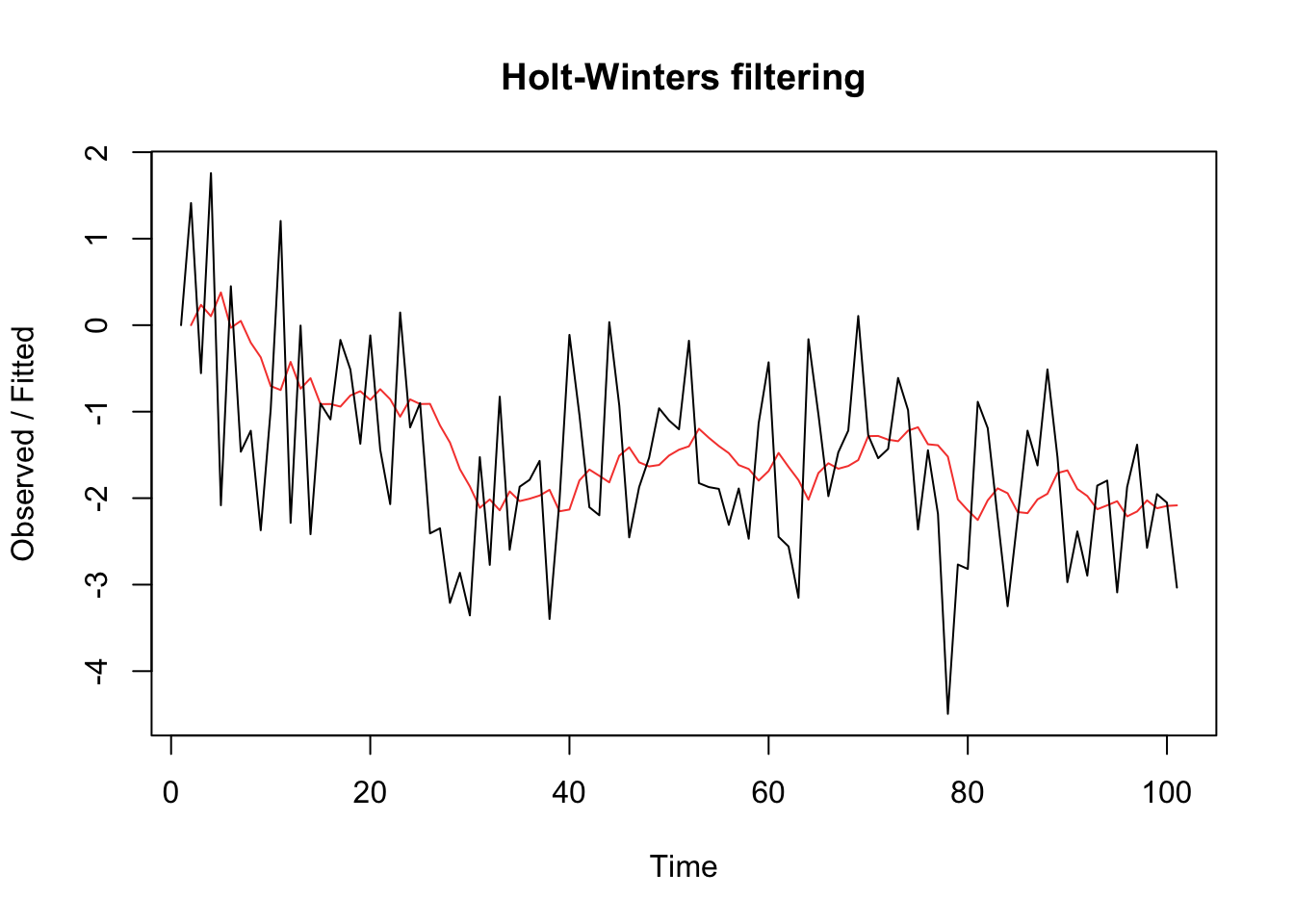
The IMA(1,1) model and exponential smoothing #

IMA(1,1) and EWMA #

• The \(ARIMA(0,1,1)\), or \(\alert{IMA(1,1)}\) model is of interest because many economic time series can be successfully modelled this way.
• The model leads to a frequently used— and abused! —forecasting method called exponentially weighted moving averages (EWMA) (“exponential smoothing” in S6).
• One should not use this method unless there is strong statistical evidence that this is the right model to use!
  (as per the following sections)

EWMA example #

set.seed(666)
x <- arima.sim(list(order = c(0, 1, 1), ma = -0.8), n = 100)  #simulate IMA(1,1)
x.ima <- HoltWinters(x, beta = FALSE, gamma = FALSE)  # fit EWMA
plot(x.ima)

Multiplicative seasonal ARIMA models (TS 3.9) #

Introduction #

• We observed seasonality in many time series so far. This is manifested when the dependence on the past tends to occur most strongly at multiples of some underlying seasonal lag \(s\). For example:
  • monthly economic data: strong yearly component occurring at lags that are multiples of \(s = 12\);
  • data taken quarterly: will exhibit the yearly repetitive period at \(s = 4\) quarters.
• In this section, we introduce several modifications made to the ARIMA model to account for seasonal and nonstationary behavior.
• The reference for this section is TS 3.9.
• Note that seasonality can be due to:
  • Deterministic reasons: include in trend
  • Stochastic dependence at seasonal lags \(s\): use SARIMA models

Pure seasonal \(ARMA(P,Q)_s\) models #

The pure seasonal autoregressive moving average model \(\alert{ARMA(P,Q)_s}\) takes the form $$\varPhi_P(B^s)x_t=\varTheta_Q(B^s)w_t,$$ where $$ \varPhi_P(B^s) = 1-\varPhi_1 B^s-\varPhi_2 B^{2s}-\cdots-\varPhi_P B^{Ps}$$ is the seasonal autoregressive operator of order \(\alert{P}\) with seasonal period \(\alert{s}\), and where $$ \varTheta_Q(B^s) = 1+\varTheta_1 B^s+\varTheta_2 B^{2s}+\cdots+\varTheta_Q B^{Ps}$$ is the seasonal moving average operator of order \(\alert{Q}\) with seasonal period \(\alert{s}\).

Here, inter-temporal correlations are exclusively seasonal (there are no non-seasonal correlations).

Note: (analogous to nonseasonal ARMA)

• It will be causal only when the roots of \(\varPhi_P(z^s)\) lie outside the unit circle
• It will be invertible only when the roots of \(\varTheta_Q(z^s)\) lie outside the unit circle

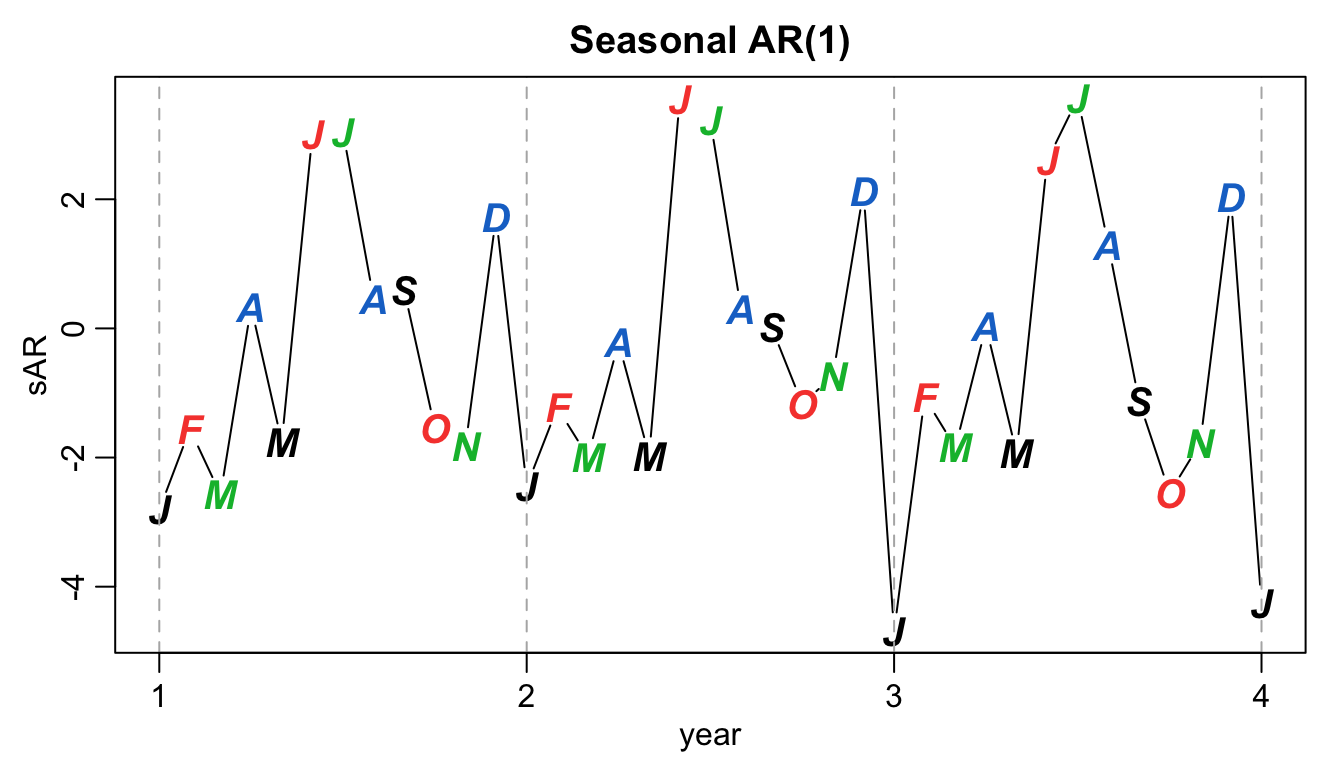
Example: first order seasonal \((s=12)\) AR model #

A first-order seasonal autoregressive series that might run over months could be written as $$ \left(1-\varPhi B^{12}\right)x_t = w_t \quad\quad \text{or} \quad\quad x_t = \varPhi x_{t-12}+w_t.$$` Note:

• \(x_t\) is expressed in terms of past lags at multiple of the (yearly) seasonal period \(s=12\) months
• very similar to the unit lag model \(AR(1)\) that we know
• causal if \(|\varPhi|<1\)
  Simulated example (with \(\varPhi=0.9\)):

set.seed(666)
phi <- c(rep(0, 11), 0.9)
sAR <- arima.sim(list(order = c(12, 0, 0), ar = phi), n = 37)
sAR <- ts(sAR, freq = 12)

par(mar = c(3, 3, 2, 1), mgp = c(1.6, 0.6, 0))
plot(sAR, axes = FALSE, main = "Seasonal AR(1)", xlab = "year",
  type = "c")
Months <- c("J", "F", "M", "A", "M", "J", "J", "A", "S", "O",
  "N", "D")
points(sAR, pch = Months, cex = 1.25, font = 4, col = 1:4)
axis(1, 1:4)
abline(v = 1:4, lty = 2, col = gray(0.7))
axis(2)
box()

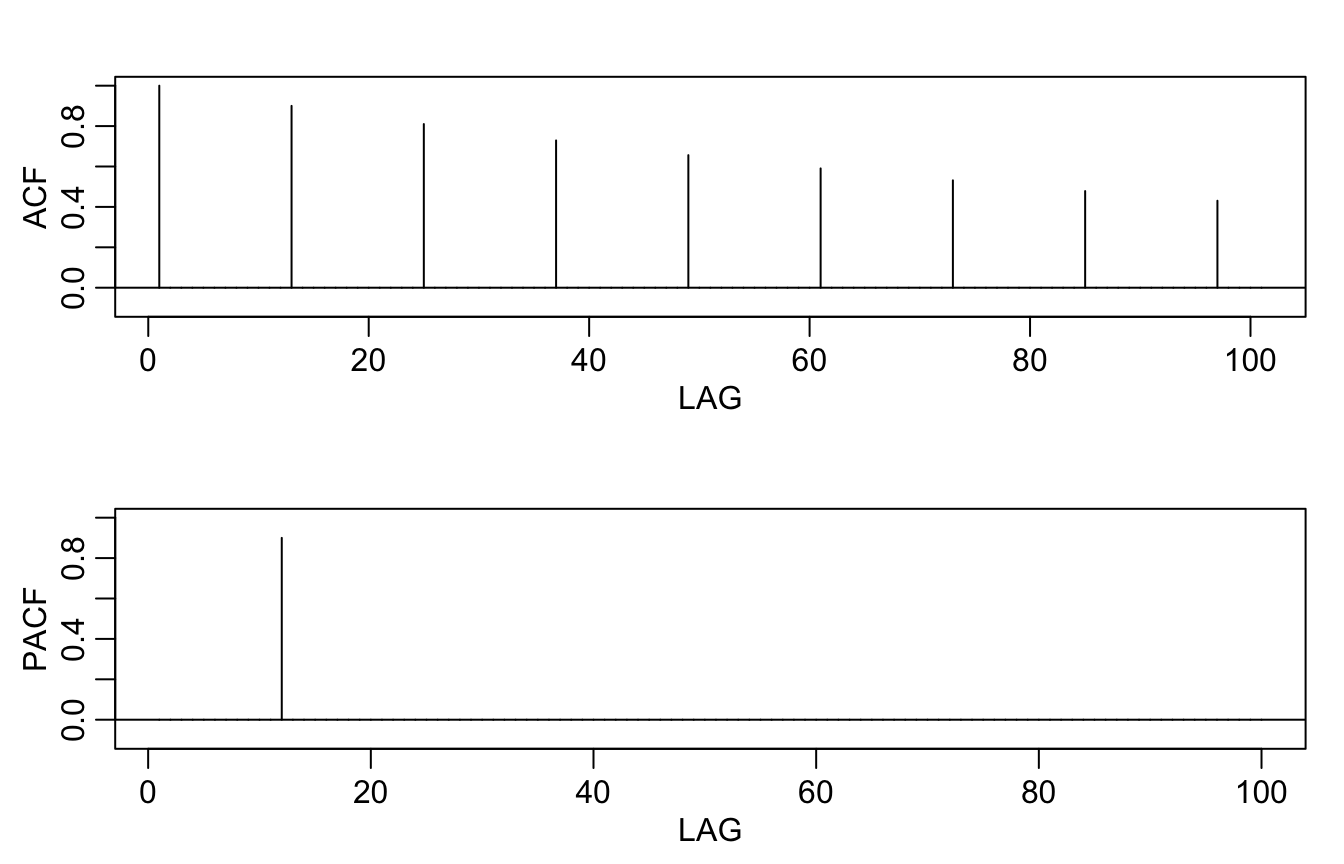
Theoretical ACF and PACF of the model:

ACF <- ARMAacf(ar = phi, ma = 0, 100)
PACF <- ARMAacf(ar = phi, ma = 0, 100, pacf = TRUE)
par(mfrow = c(2, 1), mar = c(3, 3, 2, 1), mgp = c(1.6, 0.6, 0))
plot(ACF, type = "h", xlab = "LAG", ylim = c(-0.1, 1))
abline(h = 0)
plot(PACF, type = "h", xlab = "LAG", ylim = c(-0.1, 1))
abline(h = 0)

Autocovariance and ACF of first-order seasonal models #

1. For the first-order seasonal \((s=12)\) MA model $$x_t=w_t+\varTheta w_{t-12}$$ we have $$\begin{array}{rcl} \gamma(0) &=& (1+\varTheta^2)\sigma^2 \\ \gamma(\pm 12) &=& \varTheta \sigma^2 \\ \gamma(h) &=& 0, \text{ otherwise.} \end{array}$$ Thus, the only nonzero correlation (aside from lag zero) is $$\rho(\pm 12) = \frac{\varTheta}{1+\varTheta^2}.$$ The PACF will tail off at multiples of \(s=12\).

2. For the first-order seasonal \((s=12)\) AR model $$x_t = \varPhi x_{t-12}+w_t$$ we have $$\begin{array}{rcl} \gamma(0) &=& \frac{\sigma^2}{1-\varPhi^2} \\ \gamma(\pm 12k) &=& \frac{\sigma^2\varPhi^k}{1-\varPhi^2},\quad k=1,2,\ldots \\ \gamma(h) &=& 0, \text{ otherwise.} \end{array}$$ Thus, the only nonzero correlations are $$\rho(\pm 12k) = \varPhi^k,\quad k=1,2,\ldots.$$ The PACF will have one nonzero correlation at \(s=12\) and then cut off.

Multiplicative seasonal \(ARMA(p,q)\times(P,Q)_s\) models #

In general, we can combine the seasonal and nonseasonal operators into a multiplicative seasonal autoregressive moving average model \(\alert{ARMA(p,q)\times(P,Q)_s}\), and write $$\varPhi_P(B^s)\phi(B)x_t = \varTheta_Q(B^s)\theta(B)w_t$$ as the overall model.

Note:

• When selecting a model, we will need to carefully examine the ACF and PACF of the data.
• Choosing the seasonal autoregressive and moving average components first will generally lead to better results.
• This will be discussed more in Module 10.

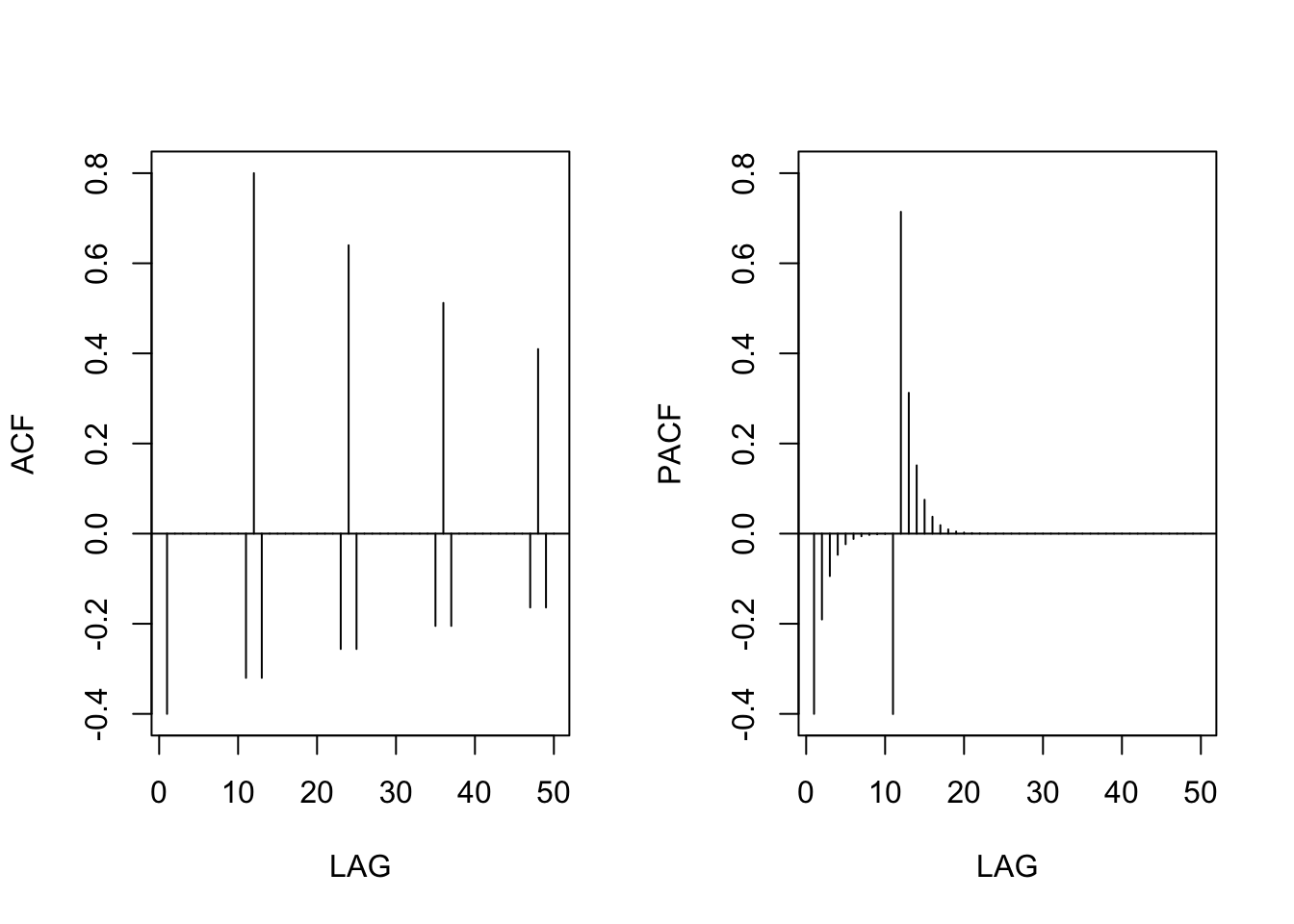
Example: A mixed seasonal model \(ARMA(0,1)\times(1,0)_{12}\) #

Consider an \(ARMA(0,1)\times(1,0)_{12}\) model $$x_t = \varPhi x_{t-12}+w_t+\theta w_{t-1},$$ where \(|\varPhi|<1\) and \(|\theta|<1\).

Because

• \(x_{t-12}\), \(w_t\) and \(w_{t-1}\) are uncorrelated; and
• \(x_t\) is stationary

then $$\gamma(0)=\varPhi^2 \gamma(0)+\sigma_w^2+\theta^2 \sigma_w^2 \Longleftrightarrow \gamma(0)=\frac{1+\theta^2}{1-\varPhi^2} \sigma_w^2.$$

Furthermore, multiplying the model by \(x_{t-h}\), \(h>0\) $$x_t x_{t-h} = \varPhi x_{t-12}x_{t-h} +w_t x_{t-h}+ \theta w_{t-1}x_{t-h}$$ and taking expectations leads to $$\begin{array}{rcl} \gamma(1) &=& \varPhi \gamma(11)+\theta \sigma_w^2 \\ \gamma(h) &=& \varPhi \gamma(h-12)\text{ for }h\ge 2. \end{array}$$ The first result stems from $$\begin{array}{rcl} \gamma(1)=E[x_t x_{t-1}] &=& E[\varPhi x_{t-12}x_{t-1}] +E[w_t x_{t-1}]+ E[\theta w_{t-1}x_{t-1}]\\ &=&\varPhi \gamma(11)+0+\theta \sigma_w^2 \end{array}$$ because $$x_{t-1}=\varPhi x_{t-13}+w_{t-1}+\theta w_{t-2}.$$ Proof of the second result is similar.

Thus, the ACF for this model (requires some algebra) is

$$\begin{array}{rcl} \rho(12h) &=& \varPhi^h, \quad h=1,2,\ldots \\ \rho(12h-1) &=& \rho(12h+1)=\frac{\theta}{1+\theta^2}\varPhi^h, \quad h=0,1,2,\ldots \\ \rho(h)&=&0 \quad\text{otherwise}. \end{array}$$

Example: if \(\varPhi=0.8\) and \(\theta=-.5\), then theoretical ACF and PACF become

phi <- c(rep(0, 11), 0.8)
ACF <- ARMAacf(ar = phi, ma = -0.5, 50)[-1]  # [-1] removes 0 lag
PACF <- ARMAacf(ar = phi, ma = -0.5, 50, pacf = TRUE)
par(mfrow = c(1, 2))
plot(ACF, type = "h", xlab = "LAG", ylim = c(-0.4, 0.8))
abline(h = 0)
plot(PACF, type = "h", xlab = "LAG", ylim = c(-0.4, 0.8))
abline(h = 0)

Seasonal differencing #

Motivating example #

• Consider average temperatures over the years.
• Each January would be approximately the same (as would February, etc…).
• In this case we might think of the average monthly temperature as $$x_t = S_t+w_t,$$ where \(S_t\) is a seasonal component that varies a little from one year to the next, say (random walk) $$S_t=S_{t-12}+v_t.$$
• Here, \(v_t\) and \(w_t\) are uncorrelated white noise processes.

• Note $$ x_{t}=S_{t-12}+v_t+w_t \text{ and } x_{t-12}= S_{t-12}+w_{t-12}.$$
• If we subtract the effect of successive years from each other (“seasonal differencing”), we find that $$(1-B^{12})x_t=x_t-x_{t-12}=v_t+w_t-w_{t-12}.$$
• This model is a stationary purely seasonal \(MA(1)_{12}\), and its ACF will have a peak only at lag 12.
• Such a model would exhibit an ACF that is large and decays very slowly at lags \(h=12k\), for \(k=1,2,\ldots\).

Seasonal differencing #

• In general, seasonal differencing can be indicated when the ACF decays slowly at multiples of some season \(s\), but is negligible between the periods.
• The seasonal difference of order \(D\) is defined as $$\nabla_s^D x_t = (1-B^s)^D x_t,$$ where \(D=1,2,\ldots\) takes positive integer values
• Typically, \(D=1\) is sufficient to obtain seasonal stationarity

How do we combine this idea with an ARIMA model?

SARIMA model \(ARIMA(p,d,q)\times(P,D,Q)_s\) #

The multiplicative seasonal autoregressive integrated moving average model, or SARIMA model is given by $$\textcolor{green}{\varPhi_P(B^s)}\textcolor{blue}{\phi(B)}\textcolor{green}{\nabla_s^D}\textcolor{blue}{\nabla^d} x_t = \delta + \textcolor{green}{\Theta_Q(B^s)}\textcolor{blue}{\theta(B)}w_t,$$ where \(w_t\) is the (usual) Gaussian white noise process.

Note:

• This is denoted as \(ARIMA\textcolor{blue}{(p,d,q)}\times\textcolor{green}{(P,D,Q)_s}\).
• The ordinary autoregressive and moving average components are represented by polynomials \(\textcolor{blue}{\phi(B)}\) and \(\textcolor{blue}{\theta(B)}\) of orders \(\textcolor{blue}{p}\) and \(\textcolor{blue}{q}\), respectively.
• The seasonal autoregressive and moving average components by \(\textcolor{green}{\varPhi_P(B^s)}\) and \(\textcolor{green}{\varTheta_Q(B^s)}\) of orders \(\textcolor{green}{P}\) and \(\textcolor{green}{Q}\), respectively.
• The ordinary and seasonal difference components by
  \(\textcolor{blue}{\nabla^d =(1-B)^d}\) and \(\textcolor{green}{\nabla_s^D =(1-B^s)^D}\).

A typical SARIMA model #

Consider the following \(ARIMA(0, 1, 1)\times(0, 1, 1)_{12}\) model with seasonal fluctuations that occur every 12 months, $$\nabla_{12}\nabla x_t = \varTheta(B^{12})\theta(B)w_t,$$ where we have set \(\delta=0\).

Note:

• This model often provides a reasonable representation for seasonal, nonstationary, economic time series.
• This model can be represented equivalently as $$\begin{array}{rcl} (1-B^{12})(1-B)x_t &=&(1+\varTheta B^{12})(1+\theta B)w_t \\ (1-B-B^{12}+B^{13})x_t &=& (1+\theta B + \varTheta B^{12}+\varTheta \theta B^{13})w_t. \end{array}$$

Yet another representation is $$x_t = x_{t-1}+x_{t-12}-x_{t-13}+w_t+\theta w_{t-1}+\varTheta w_{t-12}+\varTheta \theta w_{t-13}.$$

• The multiplicative nature implies that the coefficient of \(w_{t-13}\) is \(\varTheta \theta\) rather than yet another free parameter.
• However, this often works well, and reduces the number of parameters needed.

Example: Air Passengers #

Consider the R data set AirPassengers, which are the monthly totals of international airline passengers, 1949 to 1960, taken from Box & Jenkins (1970):

x <- AirPassengers

We’ll explore this dataset and see we can “difference out” some seasonality.

Let’s have a look at the series:

plot.ts(x, main = "Air Passengers series, unmodified")

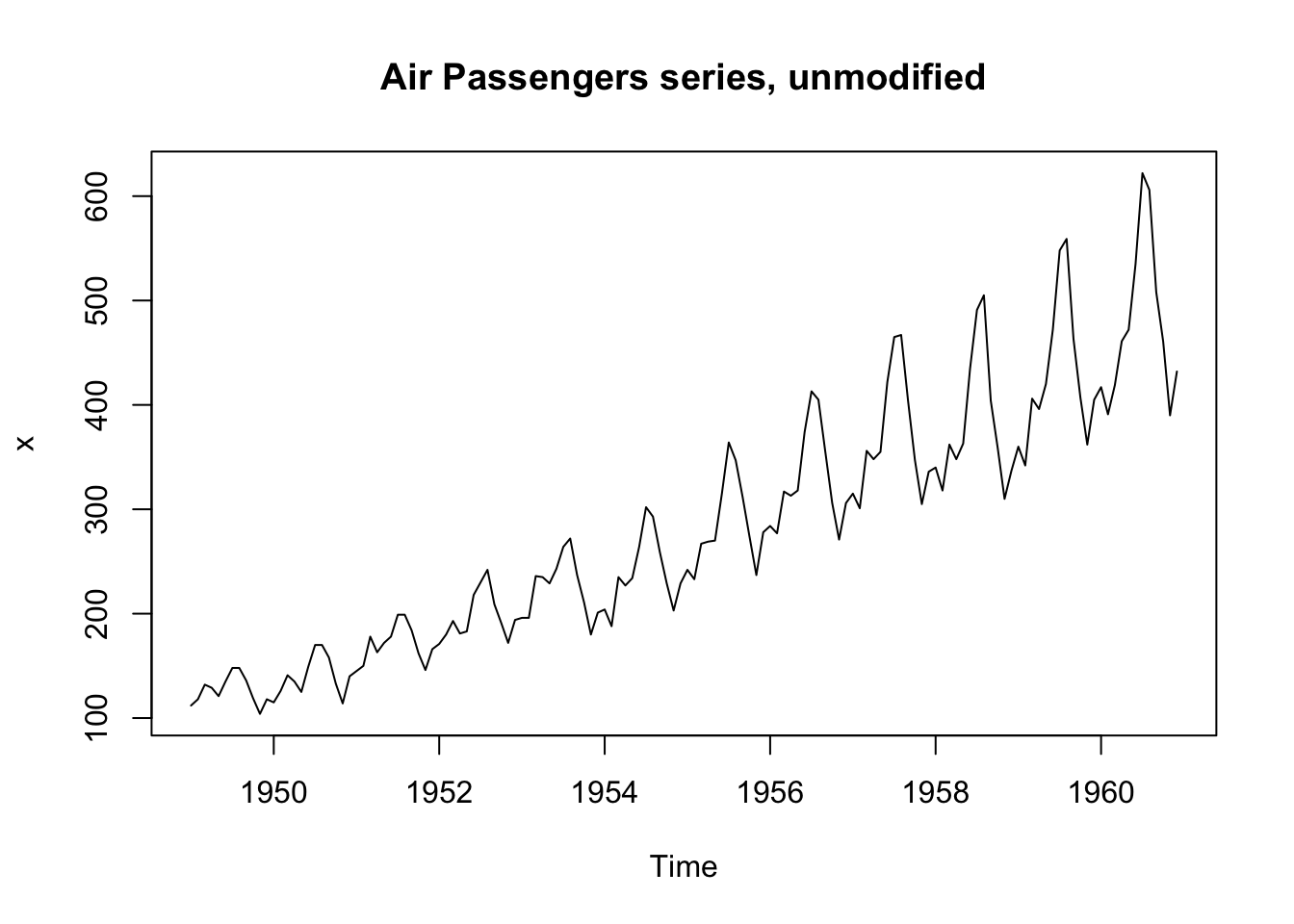
This shows trend plus increasing variance \(\rightarrow\) try a log transformation.

lx <- log(x)
plot.ts(lx, main = "Log of Air Passengers series")

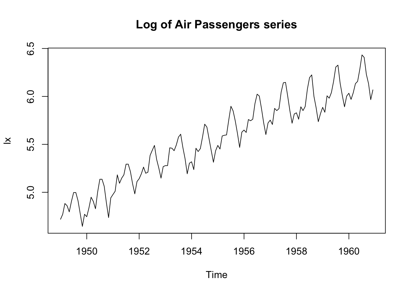
The log transformation has stabilised the variance.

We now need to remove the trend, and try differencing:

dlx <- diff(lx)
plot.ts(dlx, main = "Differenced Log of Air Passengers series")

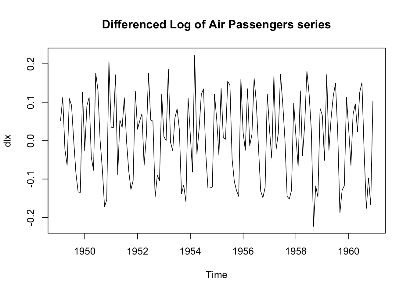
It is clear that there is still persistence in the seasons, that is,
dlx$t\approx;$ dlx${t-12}$.

We apply a twelvth-order difference:

ddlx <- diff(dlx, 12)
plot.ts(ddlx, main = "[s=12]-differenced Differenced Log of Air Passengers series")

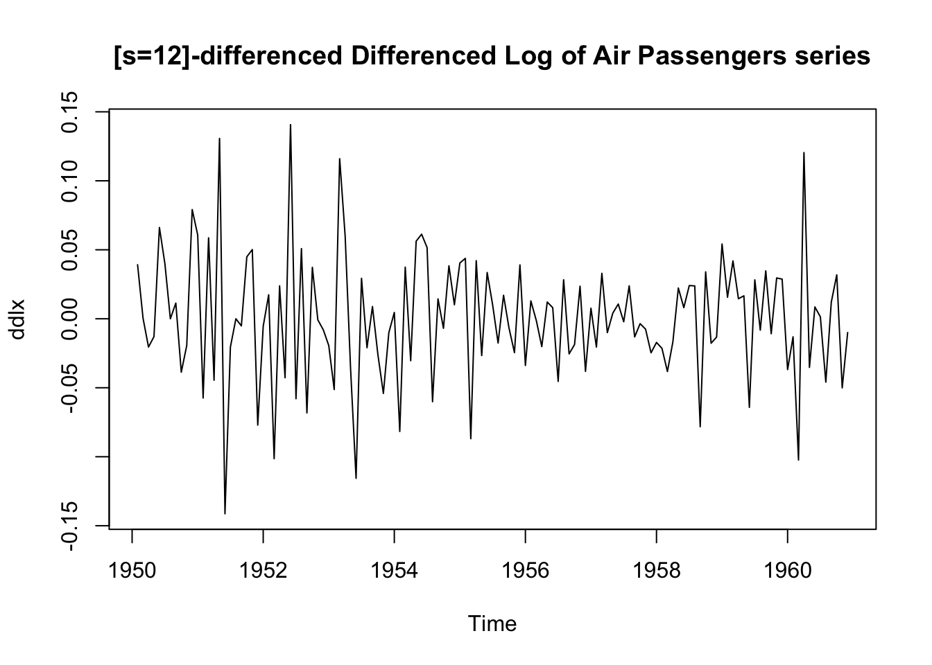
This seems to have removed the seasonality:

par(mfrow = c(2, 1), mar = c(3, 3, 2, 1), mgp = c(1.6, 0.6, 0))
monthplot(dlx)
monthplot(ddlx)

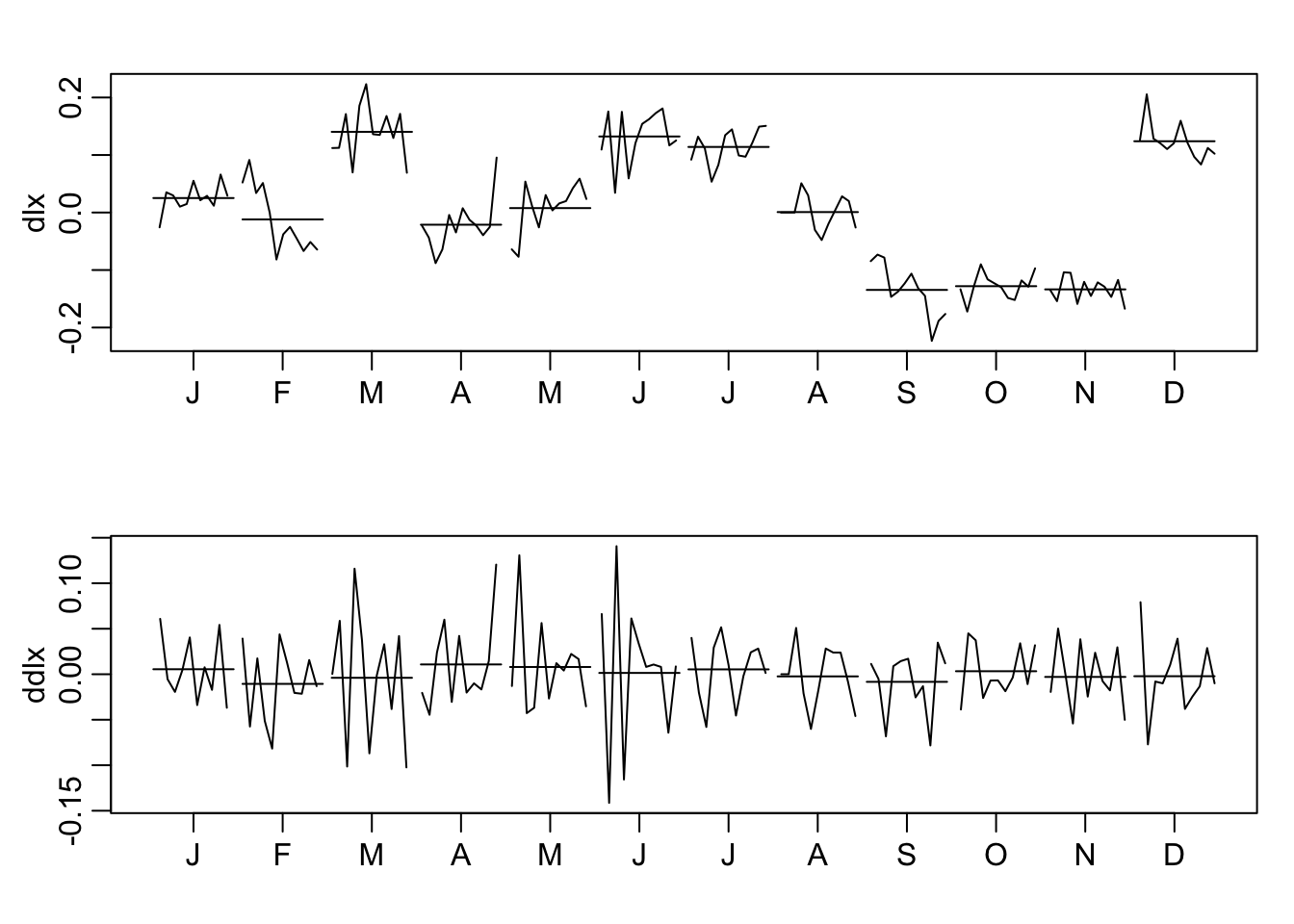
Note the monthplot function.

To summarise:

plot.ts(cbind(x, lx, dlx, ddlx), main = "")

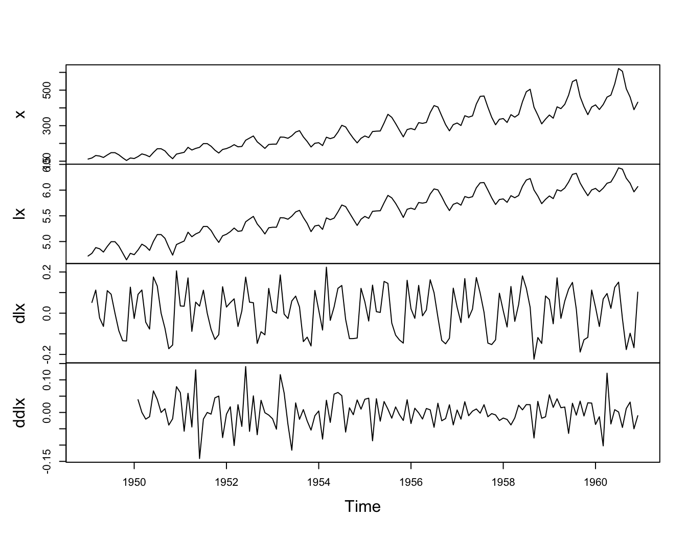
The transformed data appears to be stationary and
we are now ready to fit a model (see Module 10).

Multivariate time series (TS 5.6) #

Introduction #

• Many data sets involve more than one time series, and we are often interested in the possible dynamics relating all series.
• We are thus interested in modelling and forecasting \(k\times 1\) vector-valued time series $$x_t=(x_{t1},\ldots,x_{tk})',\quad t=0,\pm1,\pm2,\ldots.$$
• Unfortunately, extending univariate ARMA models to the multivariate case is not so simple.
• The multivariate autoregressive model, however, is a straight-forward extension of the univariate AR model.
• The resulting models are called Vector Auto-Regressive (VAR) models.
• The reference for this section is TS 5.6.

VAR(1) model #

For the first-order vector autoregressive model, VAR(1), we take $$x_t =\alpha+\Phi x_{t-1}+w_t,$$ where \(\Phi\) is a \(k\times k\) transition matrix that expresses the dependence of \(x_t\) on \(x_{t-1}\) (note these are vectors). The vector white noise process \(w_t\) is assumed to be multivariate normal with mean-zero and covariance matrix $$E\left[ w_t w_t'\right] = \Sigma_w.$$ The vector \(\alpha = (\alpha_1, \alpha_2, . . . , \alpha_k )'\) is similar to a constant in a regression setting. If \(E[x_t] = \mu\), then \(\alpha = (I-\Phi)\mu\) as before.

Example: Mortality, Temperature, Pollution #

• Define $$x_t=(x_{t1},x_{t2},x_{t3})'$$ as a vector of dimension \(k=3\) for cardiovascular mortality \(x_{t1}\), temperature \(x_{t2}\), and particulate levels \(x_{t3}\).
• We might envision dynamic relations with first order relation $$\begin{array}{rcl} x_{t1}&=& \textcolor{blue}{\alpha_1+\beta_1 t} +\textcolor{green}{\phi_{11}}x_{t-1,1}+\textcolor{green}{\phi_{12}}x_{t-1,2}+\textcolor{green}{\phi_{13}}x_{t-1,3}+\textcolor{magenta}{w_{t1}} \\ x_{t2}&=& \textcolor{blue}{\alpha_2+\beta_2 t} +\textcolor{green}{\phi_{21}}x_{t-1,1}+\textcolor{green}{\phi_{22}}x_{t-1,2}+\textcolor{green}{\phi_{23}}x_{t-1,3}+\textcolor{magenta}{w_{t2}} \\ x_{t3}&=& \textcolor{blue}{\alpha_3+\beta_3 t} +\textcolor{green}{\phi_{31}}x_{t-1,1}+\textcolor{green}{\phi_{32}}x_{t-1,2}+\textcolor{green}{\phi_{33}}x_{t-1,3}+\textcolor{magenta}{w_{t3}} \end{array}$$
• This can be rewritten in matrix form as $$x_t=\textcolor{blue}{\Gamma u_t} +\textcolor{green}{\Phi} x_{t-1}+\textcolor{magenta}{w_t},$$ where \(\Gamma=[\alpha|\beta]\) is \(3\times 2\) and \(u_t=(1,t)'\) is \(2x1\).

We use the R package vars to fit VAR models via least squares.

library(vars)
x <- cbind(cmort, tempr, part)
summary(VAR(x, p = 1, type = "both"))  # 'both' fits constant + trend
...
## VAR Estimation Results:
## ========================= 
## Endogenous variables: cmort, tempr, part 
## Deterministic variables: both 
## Sample size: 507 
## Log Likelihood: -5116.02 
## Roots of the characteristic polynomial:
## 0.8931 0.4953 0.1444
## Call:
## VAR(y = x, p = 1, type = "both")
...

Note that roots less than one here ensure stability; see this

library(vars)
x <- cbind(cmort, tempr, part)
summary(VAR(x, p = 1, type = "both"))  # 'both' fits constant + trend
...
## Estimation results for equation cmort: 
## ====================================== 
## cmort = cmort.l1 + tempr.l1 + part.l1 + const + trend 
## 
##           Estimate Std. Error t value Pr(>|t|)    
## cmort.l1  0.464824   0.036729  12.656  < 2e-16 ***
## tempr.l1 -0.360888   0.032188 -11.212  < 2e-16 ***
## part.l1   0.099415   0.019178   5.184 3.16e-07 ***
## const    73.227292   4.834004  15.148  < 2e-16 ***
## trend    -0.014459   0.001978  -7.308 1.07e-12 ***
## ---
## Signif. codes:  0 '***' 0.001 '**' 0.01 '*' 0.05 '.' 0.1 ' ' 1
## 
## 
## Residual standard error: 5.583 on 502 degrees of freedom
## Multiple R-Squared: 0.6908,	Adjusted R-squared: 0.6883 
## F-statistic: 280.3 on 4 and 502 DF,  p-value: < 2.2e-16 
...

library(vars)
x <- cbind(cmort, tempr, part)
summary(VAR(x, p = 1, type = "both"))  # 'both' fits constant + trend
...
## Estimation results for equation tempr: 
## ====================================== 
## tempr = cmort.l1 + tempr.l1 + part.l1 + const + trend 
## 
##           Estimate Std. Error t value Pr(>|t|)    
## cmort.l1 -0.244046   0.042105  -5.796 1.20e-08 ***
## tempr.l1  0.486596   0.036899  13.187  < 2e-16 ***
## part.l1  -0.127661   0.021985  -5.807 1.13e-08 ***
## const    67.585598   5.541550  12.196  < 2e-16 ***
## trend    -0.006912   0.002268  -3.048  0.00243 ** 
## ---
## Signif. codes:  0 '***' 0.001 '**' 0.01 '*' 0.05 '.' 0.1 ' ' 1
## 
## 
## Residual standard error: 6.4 on 502 degrees of freedom
## Multiple R-Squared: 0.5007,	Adjusted R-squared: 0.4967 
## F-statistic: 125.9 on 4 and 502 DF,  p-value: < 2.2e-16 
...

library(vars)
x <- cbind(cmort, tempr, part)
summary(VAR(x, p = 1, type = "both"))  # 'both' fits constant + trend
...
## Estimation results for equation part: 
## ===================================== 
## part = cmort.l1 + tempr.l1 + part.l1 + const + trend 
## 
##           Estimate Std. Error t value Pr(>|t|)    
## cmort.l1 -0.124775   0.079013  -1.579    0.115    
## tempr.l1 -0.476526   0.069245  -6.882 1.77e-11 ***
## part.l1   0.581308   0.041257  14.090  < 2e-16 ***
## const    67.463501  10.399163   6.487 2.10e-10 ***
## trend    -0.004650   0.004256  -1.093    0.275    
## ---
## Signif. codes:  0 '***' 0.001 '**' 0.01 '*' 0.05 '.' 0.1 ' ' 1
## 
## 
## Residual standard error: 12.01 on 502 degrees of freedom
## Multiple R-Squared: 0.3732,	Adjusted R-squared: 0.3683 
## F-statistic: 74.74 on 4 and 502 DF,  p-value: < 2.2e-16 
...

library(vars)
x <- cbind(cmort, tempr, part)
summary(VAR(x, p = 1, type = "both"))  # 'both' fits constant + trend
...
## Covariance matrix of residuals:
##        cmort  tempr   part
## cmort 31.172  5.975  16.65
## tempr  5.975 40.965  42.32
## part  16.654 42.323 144.26
## 
## Correlation matrix of residuals:
##        cmort  tempr   part
## cmort 1.0000 0.1672 0.2484
## tempr 0.1672 1.0000 0.5506
## part  0.2484 0.5506 1.0000
...

\(VAR(p)\) models #

• It is easy to extend the VAR(1) process to higher orders (that means with correlations going farther than one step into the past), leading to \(\alert{VAR(p)}\).
• The regressors are $$(1,x_{t-1}',x_{t-2}',\ldots,x_{t-p}')'.$$
• The regression model is then $$x_t=\alpha + \sum_{j=1}^p \Phi_j x_{t-j}+w_t.$$
• The function VARselect suggests the optimal order \(p\) according to different criteria: AIC, Hannan-Quinn (similar to BIC), BIC, and Final Prediction Error (which minimises the approximate mean squared one-step-ahead prediction error).

Example: VAR(1) on Mortality, Temperature, Pollution #

VARselect(x, lag.max = 10, type = "both")
## $selection
## AIC(n)  HQ(n)  SC(n) FPE(n) 
##      9      5      2      9 
## 
## $criteria
##                   1           2           3           4           5
## AIC(n)     11.73780    11.30185    11.26788    11.23030    11.17634
## HQ(n)      11.78758    11.38149    11.37738    11.36967    11.34557
## SC(n)      11.86463    11.50477    11.54689    11.58541    11.60755
## FPE(n) 125216.91717 80972.28678 78268.19568 75383.73647 71426.10041
##                  6           7           8           9          10
## AIC(n)    11.15266    11.15247    11.12878    11.11915    11.12019
## HQ(n)     11.35176    11.38144    11.38760    11.40784    11.43874
## SC(n)     11.65996    11.73587    11.78827    11.85473    11.93187
## FPE(n) 69758.25113 69749.89175 68122.40518 67476.96374 67556.45243

We will proceed with order \(p=2\) according to BIC.

summary(fit <- VAR(x, p = 2, type = "both"))
...
## VAR Estimation Results:
## ========================= 
## Endogenous variables: cmort, tempr, part 
## Deterministic variables: both 
## Sample size: 506 
## Log Likelihood: -4987.186 
## Roots of the characteristic polynomial:
## 0.8807 0.8807 0.5466 0.4746 0.4746 0.4498
## Call:
## VAR(y = x, p = 2, type = "both")
...

summary(fit <- VAR(x, p = 2, type = "both"))
...
## Estimation results for equation cmort: 
## ====================================== 
## cmort = cmort.l1 + tempr.l1 + part.l1 + cmort.l2 + tempr.l2 + part.l2 + const + trend 
## 
##           Estimate Std. Error t value Pr(>|t|)    
## cmort.l1  0.297059   0.043734   6.792 3.15e-11 ***
## tempr.l1 -0.199510   0.044274  -4.506 8.23e-06 ***
## part.l1   0.042523   0.024034   1.769  0.07745 .  
## cmort.l2  0.276194   0.041938   6.586 1.15e-10 ***
## tempr.l2 -0.079337   0.044679  -1.776  0.07639 .  
## part.l2   0.068082   0.025286   2.692  0.00733 ** 
## const    56.098652   5.916618   9.482  < 2e-16 ***
## trend    -0.011042   0.001992  -5.543 4.84e-08 ***
## ---
## Signif. codes:  0 '***' 0.001 '**' 0.01 '*' 0.05 '.' 0.1 ' ' 1
## 
## 
## Residual standard error: 5.295 on 498 degrees of freedom
## Multiple R-Squared: 0.7227,	Adjusted R-squared: 0.7188 
## F-statistic: 185.4 on 7 and 498 DF,  p-value: < 2.2e-16 
...

summary(fit <- VAR(x, p = 2, type = "both"))
...
## Estimation results for equation tempr: 
## ====================================== 
## tempr = cmort.l1 + tempr.l1 + part.l1 + cmort.l2 + tempr.l2 + part.l2 + const + trend 
## 
##           Estimate Std. Error t value Pr(>|t|)    
## cmort.l1 -0.108889   0.050667  -2.149  0.03211 *  
## tempr.l1  0.260963   0.051292   5.088 5.14e-07 ***
## part.l1  -0.050542   0.027844  -1.815  0.07010 .  
## cmort.l2 -0.040870   0.048587  -0.841  0.40065    
## tempr.l2  0.355592   0.051762   6.870 1.93e-11 ***
## part.l2  -0.095114   0.029295  -3.247  0.00125 ** 
## const    49.880485   6.854540   7.277 1.34e-12 ***
## trend    -0.004754   0.002308  -2.060  0.03993 *  
## ---
## Signif. codes:  0 '***' 0.001 '**' 0.01 '*' 0.05 '.' 0.1 ' ' 1
## 
## 
## Residual standard error: 6.134 on 498 degrees of freedom
## Multiple R-Squared: 0.5445,	Adjusted R-squared: 0.5381 
## F-statistic: 85.04 on 7 and 498 DF,  p-value: < 2.2e-16 
...

summary(fit <- VAR(x, p = 2, type = "both"))
...
## Estimation results for equation part: 
## ===================================== 
## part = cmort.l1 + tempr.l1 + part.l1 + cmort.l2 + tempr.l2 + part.l2 + const + trend 
## 
##           Estimate Std. Error t value Pr(>|t|)    
## cmort.l1  0.078934   0.091773   0.860 0.390153    
## tempr.l1 -0.388808   0.092906  -4.185 3.37e-05 ***
## part.l1   0.388814   0.050433   7.709 6.92e-14 ***
## cmort.l2 -0.325112   0.088005  -3.694 0.000245 ***
## tempr.l2  0.052780   0.093756   0.563 0.573724    
## part.l2   0.382193   0.053062   7.203 2.19e-12 ***
## const    59.586169  12.415669   4.799 2.11e-06 ***
## trend    -0.007582   0.004180  -1.814 0.070328 .  
## ---
## Signif. codes:  0 '***' 0.001 '**' 0.01 '*' 0.05 '.' 0.1 ' ' 1
## 
## 
## Residual standard error: 11.11 on 498 degrees of freedom
## Multiple R-Squared: 0.4679,	Adjusted R-squared: 0.4604 
## F-statistic: 62.57 on 7 and 498 DF,  p-value: < 2.2e-16 
...

summary(fit <- VAR(x, p = 2, type = "both"))
...
## Covariance matrix of residuals:
##        cmort  tempr   part
## cmort 28.034  7.076  16.33
## tempr  7.076 37.627  40.88
## part  16.325 40.880 123.45
## 
## Correlation matrix of residuals:
##        cmort  tempr   part
## cmort 1.0000 0.2179 0.2775
## tempr 0.2179 1.0000 0.5998
## part  0.2775 0.5998 1.0000
...

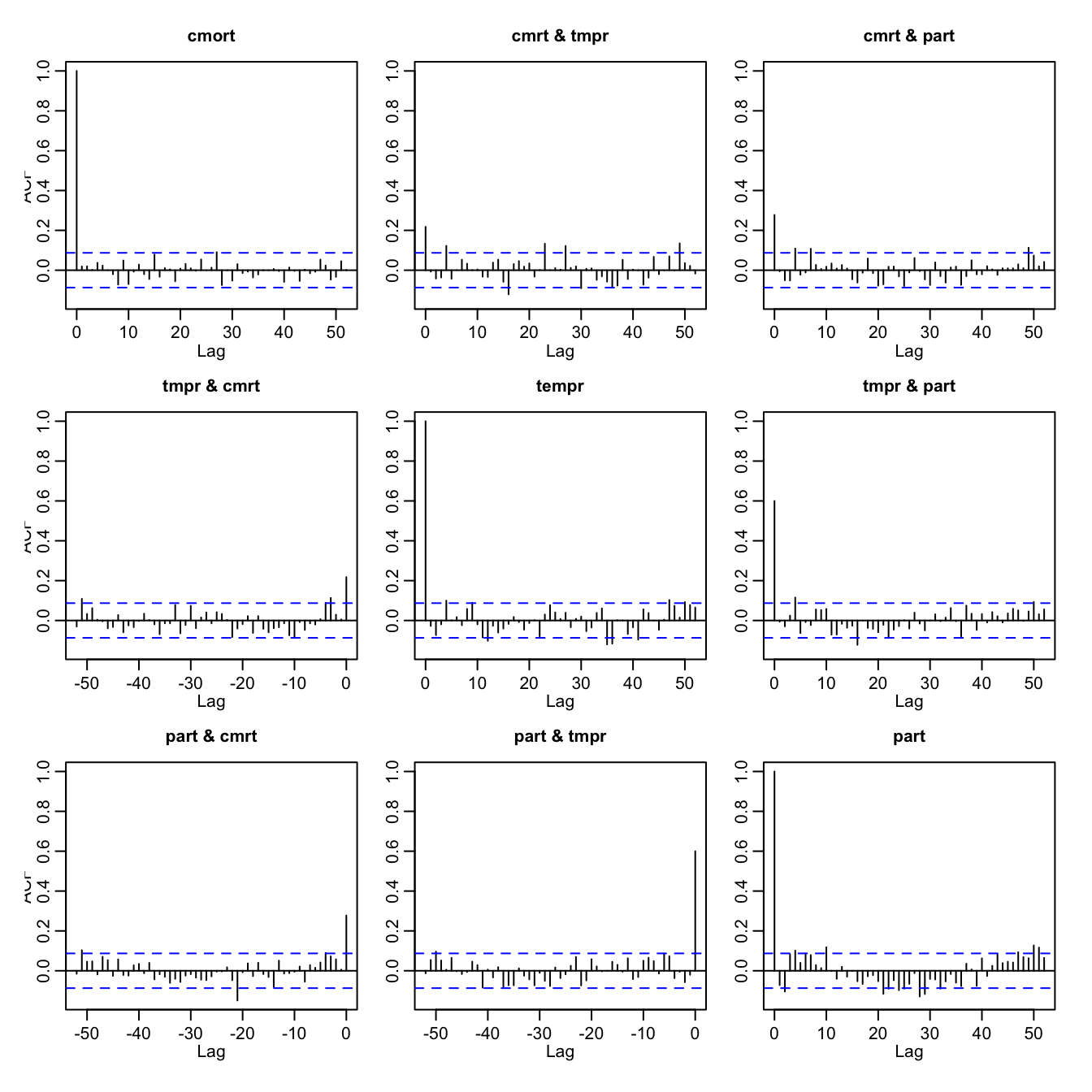
Furthermore, the Portmanteau test rejects the null hypothesis of white noise, suggesting poor fit:

serial.test(fit, lags.pt = 12, type = "PT.adjusted")
## 
## 	Portmanteau Test (adjusted)
## 
## data:  Residuals of VAR object fit
## Chi-squared = 162.35, df = 90, p-value = 4.602e-06

This is confirmed by visual inspection:

acf(resid(fit), 52)

acf(resid(fit), 52)

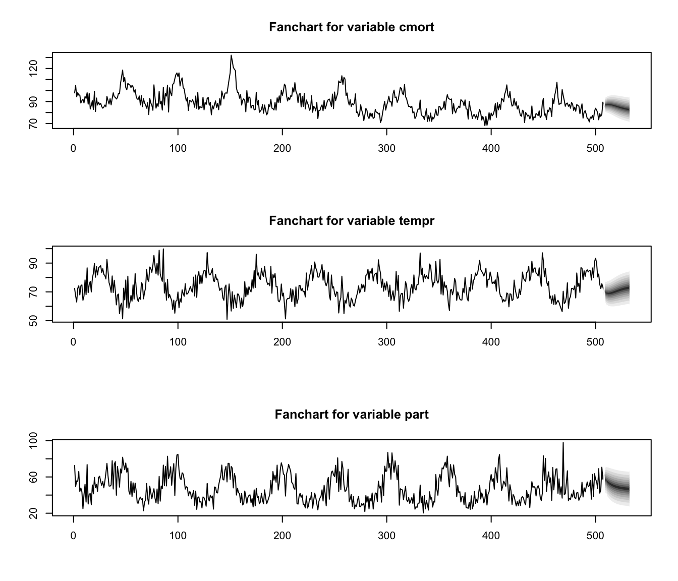
Predictions are produced with

fit.pr <- predict(fit, n.ahead = 24, ci = 0.95)  # 24 weeks ahead
fanchart(fit.pr)  # plot prediction + error

Special cases briefly mentioned in CS2 syllabus (S6) #

Bilinear models #

• Consider the bilinear model $$x_t-\alpha(x_{t-1}-\mu)=\mu+w_t+\beta w_{t-1}+b(x_t-\mu)w_{t-1}.$$
• This equation is linear in \(x_t\), and also linear in \(w_t\) - hence the name of .
• This can be rewritten as \begin{eqnarray*} x_t&=&\mu+w_t \\ &&+(\beta +b(x_t-\mu)) w_{t-1}\\ &&+\alpha(x_{t-1}-\mu). \end{eqnarray*}
• As opposed to ARMA models, the bilinear models exhibit behaviour: when the process is far from its mean it tends to exhibit larger fluctuations.
• When the process is “at” its mean, dynamics are similar
  to that of an \(MA(1)\) process.

Threshold autoregressive models #

• Consider the threshold autogressive model $$x_t=\mu+\left\{\begin{array}{lc} \alpha_1(x_{t-1}-\mu)+w_t & x_{t-1}\le d, \\ \alpha_2(x_{t-1}-\mu)+w_t & x_{t-1}> d. \end{array}\right.$$
• A distinctive feature of some models from the threshold autoregressive class is limit cycle behaviour. This makes the threshold autoregressive models potential candidates for modelling ‘cyclic’ phenomena.
• The idea is to have parameters to be allowed to change in a “regime-switching” fashion, sometimes depending on the past values of \(x_t\).
• Some additional details can be found, for instance, on Wikipedia here (not assessable).

Random coefficient autoregressive models #

• Here $$x_t=\mu+\alpha_t(x_{t-1}-\mu)+w_t,$$ where \(\{\alpha_1,\alpha_2,\ldots,\alpha_n\}\) is a sequence of independent random variables.
• Such a model could be used to represent the behaviour of an investment fund, with \(\mu=0\) and \(\alpha_t=1+i_t\) where \(i_t\) is a random rate of return.
• The extra randomness make such processes more irregular than the corresponding \(AR(1)\).

Autoregressive models with conditional heteroscedasticity #

• A feature that is frequently observed in asset price data is that a significant change in the price of an asset is often followed by a period of high volatility.
• The class of autoregressive models with conditional heteroscedasticity of order \(p\)—the \(ARCH(p)\) models —is defined by the relation $$x_t=\mu+w_t\sqrt{\alpha_0+\sum_{k=1}^p \alpha_k(x_{t-k}-\mu)^2},$$ where \(w_t \sim \text{iid N}(0,\sigma_w^2)\).
• Because of the scaling of \(w_t\) with a term that is bigger as previous values of \(x_t\) are farther from their mean \(\mu\), ARCH models go towards capturing this feature.

• If \(p=1\), the \(ARCH(1)\) model is $$x_t=\mu+w_t\sqrt{\alpha_0+\alpha(x_{t-1}-\mu)^2}.$$
• ARCH models have been used for modelling financial time series. If \(z_t\) is the price of an asset at the end of the \(t\)-th trading day, set \(x_t=\log(z_t/z_{t-1})\) (the daily return on day \(t\)).
• Note:
  • Setting all \(\alpha_k=0\), \(k=1,\ldots,p\) will “switch off” the “ARCH” behaviour, and we will be back with a white noise process of variance \(\alpha_0\) (plus constant mean \(\mu\)).
  • So what we are modelling here is purely the variance of the process \(x_t\), given its past ($p$) values.
  • If we extend the idea of conditional heteroskedasticity to an ARMA structure (rather than just AR), we get the so-called “GARCH” models.

References #