Introduction (TS 2.0) #

Motivating example #

mut <- (1:12000)/1000
wt <- rnorm(12000, 0, 1)
xt <- mut + wt
xt <- as.ts(xt, frequency = c(12))
plot(xt)
lines(mut, col = "red", lwd = 2)

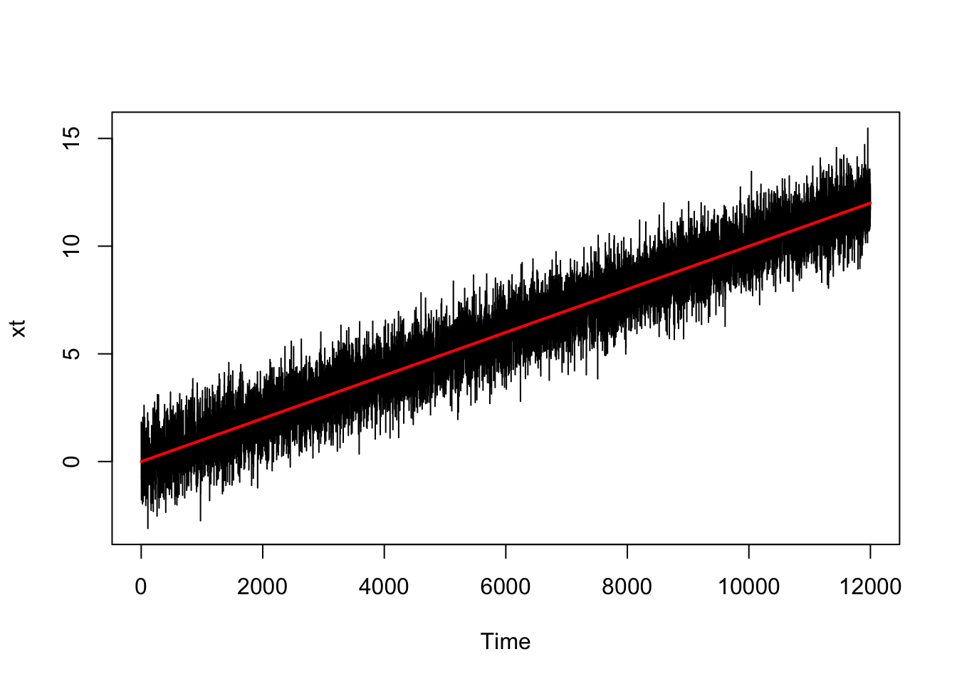
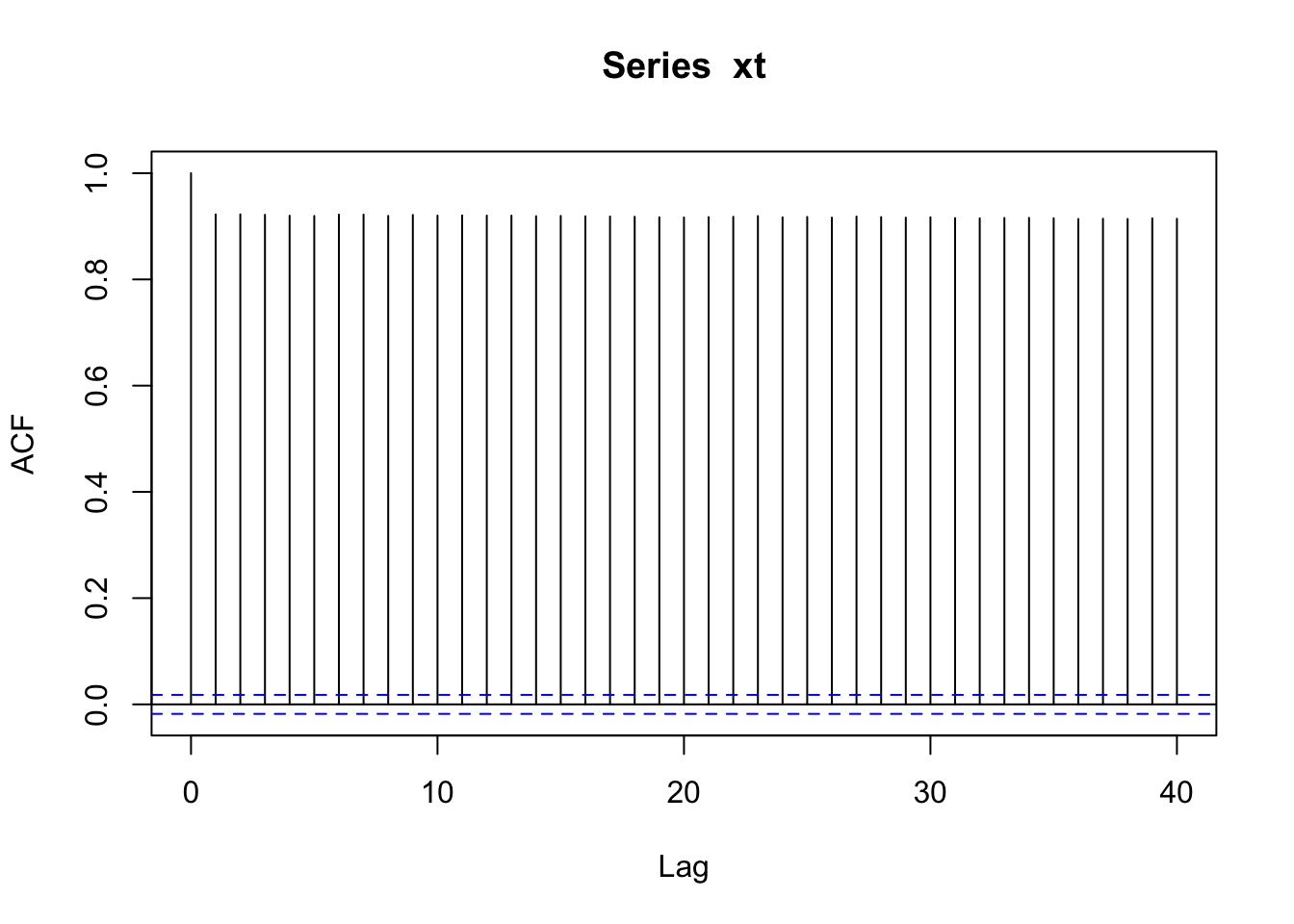
cor(xt[1:11999], xt[2:12000])

## [1] 0.9225439

cor(xt[1:11998], xt[3:12000])

## [1] 0.9228842

acf(xt)

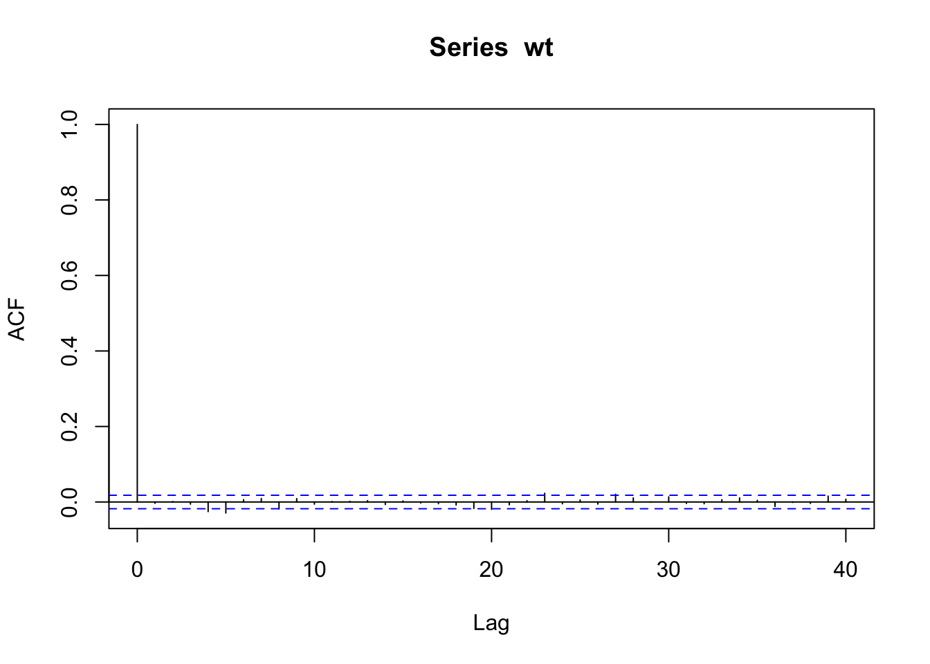
cor(wt[1:11999], wt[2:12000])

## [1] -0.003488493

cor(wt[1:11998], wt[3:12000])

## [1] 0.00116533

acf(wt)

Objectives #

• In the previous module we discussed how important it is to have stationary time series, and started to hint at methods to render time series stationary and/or white noise.
• In this module we discuss those techniques more precisely and more comprehensively.
• This includes:
  • regression in the context of time series
  • de-trending via regression
  • de-trending via differencing
  • nonparametric smoothing of time series
    (to help with the identification of trends)
• We will also introduce the backshift operator, which we will use extensively in Module 9.

Classical regression in the Time Series Context (TS 2.1) #

Regression with independent series #

Assume some output or dependent time series \(x_t\), for \(t = 1,\ldots, n\), is being influenced by a collection of \(q\) possible inputs or independent series \(z_{t1}, z_{t2},\ldots, z_{tq}\), where we first regard the inputs as fixed and known. We have then $$x_t =\beta_0+\beta_1z_{t1}+\beta_2z_{t2}+\cdots+\beta_qz_{tq}+w_t,$$ where \(\beta_0, \beta_1,\ldots, \beta_q\) are unknown fixed regression coefficients, and \(w_t \sim \text{iid N}(0,\sigma_w^2)\) Note:

• \(z_{t\cdot}\) being fixed and known is necessary for applying conventional linear regression, but we will relax this later on
• For time series regression \(w_t\) is rarely a white noise, so we will need to relax that assumption

Example: de-trending with a linear trend #

Model #

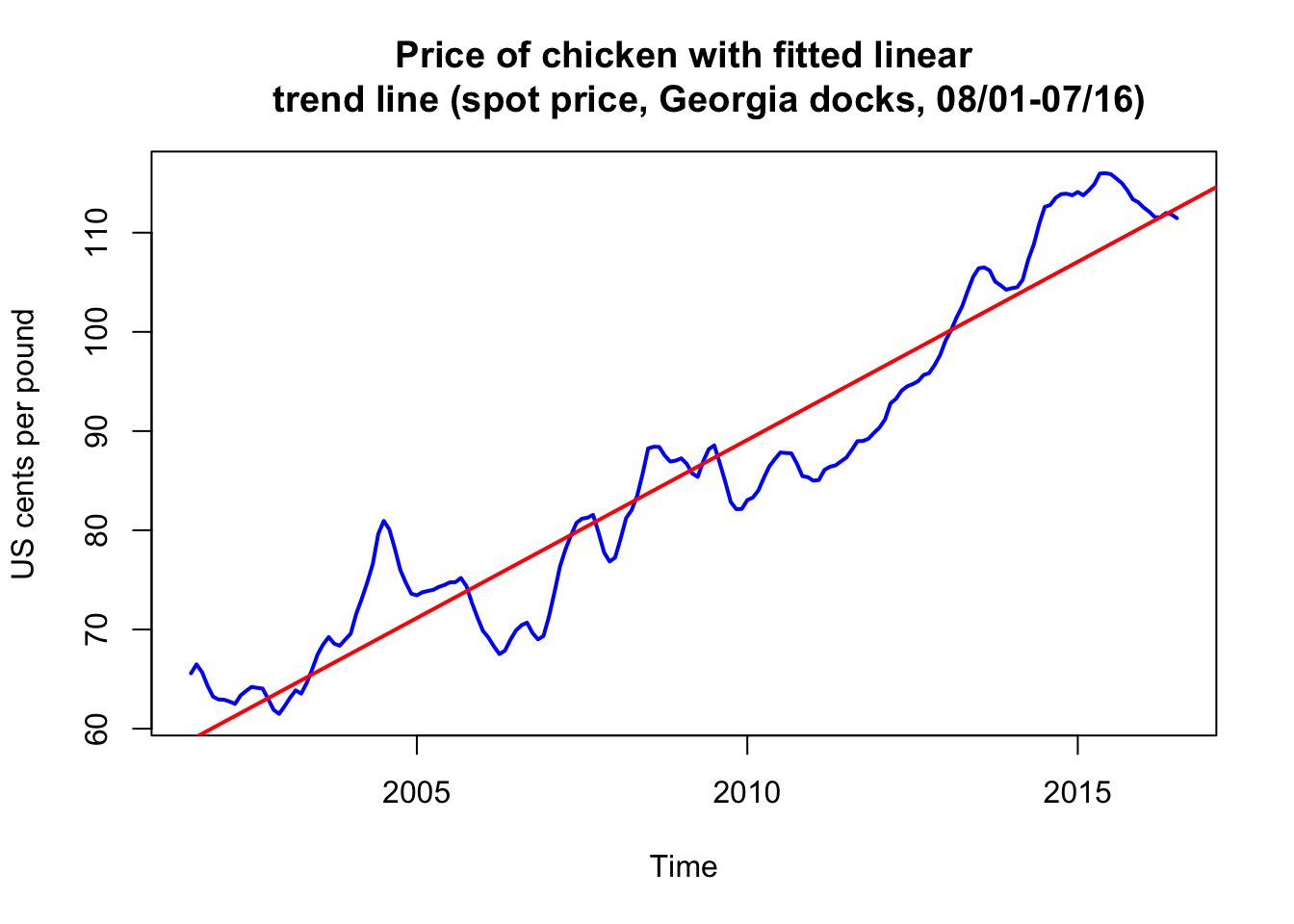
• Monthly price \(x_t\) (per pound) of a chicken in the US from mid-2001 to mid-2016 (180 months)
• We model the trend with a linear regression: $$x_t=\beta_0+\beta_1 z_t + w_t, \quad z_t=2001\frac{7}{12},2001\frac{8}{12},\ldots,2016\frac{6}{12},$$ where \(z_t\) are months in the data. Note here \(q=1\).
• Note underlying assumption are that \(w_t\sim \text{iid N}(0,\sigma_w^2)\) (uncorrelated), which may not be true.

summary(fit <- lm(chicken ~ time(chicken), na.action = NULL))

...
## Coefficients:
##                 Estimate Std. Error t value Pr(>|t|)    
## (Intercept)   -7.131e+03  1.624e+02  -43.91   <2e-16 ***
## time(chicken)  3.592e+00  8.084e-02   44.43   <2e-16 ***
## ---
## Signif. codes:  0 '***' 0.001 '**' 0.01 '*' 0.05 '.' 0.1 ' ' 1
...

• This means that \(\hat{\beta}_1=3.59\) with standard error of 0.081 (increase of about 3.6 cents per year)

Fitting results #

plot(chicken, ylab = "US cents per pound", col = "blue", lwd = 2,
  main = "Price of chicken with fitted linear
     trend line (spot price, Georgia docks, 08/01-07/16)")
abline(fit, col = "red", lwd = 2)  # add the fitted line

Revisions: Regression #

General set-up #

The multiple linear regression model written earlier can be written using vectors \(z_t=(1,z_{t},z_{t2},\ldots,z_{tq})'\) and \(\beta=(\beta_0,\beta_1,\ldots,\beta_q)'\): $$x_t =\beta_0+\beta_1z_{t1}+\beta_2z_{t2}+\cdots+\beta_qz_{tq}+w_t=\beta'z_t + w_t.$$ Parameters estimates \(\widehat{\beta}\) are obtained via ordinary least squares (OLS), that is, we minimise $$Q=\sum_{t=1}^n\left(x_t-\beta'z_t\right)^2=\sum_{t=1}^n w_t ^2$$

$$\text{with resulting minimum }\quad SSE=\sum_{t=1}^n\left(x_t-\widehat{\beta}'z_t\right)^2,$$ called sum of squares.

Properties of \(\hat{\beta}\) #

• Estimator \(\widehat{\beta}\) is unbiased and has the smallest variance within the class of linear unbiased estimators

If \(w_t\) are normally distributed:

• \(\widehat{\beta}\) also normally distributed with mean \(\beta\) and variance-covariance matrix $$Cov(\widehat{\beta})=\sigma_w^2 C, \quad C=\left(\sum_{t=1}^n z_tz_t'\right)^{-1}.$$
• Denote \(c_{ii}\) as the \(i\)-th diagonal element of \(C\).

If \(w_t\) are normally distributed and \(\sigma_w^2\) needs to be estimated:

• the distribution of \(\widehat{\beta}\) changes to a t-distribution. In this case, $$\text{t}=\frac{\widehat{\beta}_i-\beta_i}{s_w\sqrt{c_{ii}}} \sim \text{t distributed}(n-(q+1)),$$ where $$s_w^2 = \frac{SSE}{n-(q+1)}= MSE$$ is an unbiased estimator for \(\sigma_w^2\), called also mean squared error (MSE).

• This means we can construct of hypothesis test of type \(H_0:\;\beta_i=0,\) \(i=1,\ldots,q\).

Stepwise multiple regression #

Revisions: select \(z_{ti}\) through \(\widehat{\beta}\) #

• The question of model selection boils down to
  • how many independent variables \((q)\) to use?
  • which independent variables \((z_{ti})\) to use?
• Strategy is to test for statistical significance of the \(\beta_i\)’s: is there statistical evidence that \(\beta_i\) is different from 0?
• This can be done for a given independent variable \(i\), but this approach can prove tedious in practice:
  • the statistical significance of a given \(\beta_i\) changes once others are added / removed (as they may be correlated)
  • so if you have \(q\) variables, answering the two questions above with an exhaustive analysis requires testing \(q!+(q-1)!+\cdots+1\) models (quite a lot!)
• Hence, we often compare a smaller number of models, and perform tests by comparing model performance in a pairwise fashion.
• This is called stepwise multiple regression.

Process #

Consider:

• Two models of different sizes for the same data, one with \(r\) parameters, and the other with \(q>r\) parameters
• Furthermore, the original \(r\) parameters are all included in the wider set of \(q\) parameters (the smaller model is “nested” within the larger one)

Were improvements introduced by the extra \(q-r\) variables in the larger model statistically significant?

• This is done by comparing the sum of squares between the reduced model ( \(SSE_r\), with \(r\) parameters) and the original sum of squares ( \(SSE\), with \(q\) parameters).

We have that $$F=\frac{(SSE_r-SSE)/(q-r)}{SSE/(n-q-1)}\equiv\frac{MSR}{MSE}\sim F-\text{distribution}(q-r,n-q-1).$$

Results are summarised in an Analysis of Variance (ANOVA) table

• Such an output is generated by the R function aov, which outputs \(p\)-values for \(F\) and significance levels.
• If \(r=0\) the reduced model is \(x_t=\beta_0+w_t\) and the ratio $$R^2 = \frac{SSE_0-SSE}{SSE_0}$$ is called the coefficient of determination, which is one measure of the proportion of variation explained by all \(q\) variables.

Model selection #

Motivation #

Note that stepwise regression presents some issues:

• There are a lot of paths from the null \((q=0)\) to the full \((q=n)\) model, and it is not always clear which ones to investigate first, and there can be a lot of trial and error
• One can compare only nested models - what if we want to compare with models of a different nature?
• Asymptotic results behind the hypothesis tests that are used pre-suppose normality of the errors, which is not always correct.

What if one wanted to assess models based on their own merits, rather than sequentially? This leads to the idea of information criteria. These balance the concepts of

• likelihood (the more parameters the better), and
• parsimony, represented by the number of parameters
  (the least parameters the better).

Preliminary #

First, note that the maximum likelihood estimator for the variance is $$\hat{\sigma}_k^2=\frac{SSE(k)}{n},$$ where \(SSE(k)\) denotes the residual sum of squares under the model with \(k\) regression coefficients, and where \(n\) is the sample size.

Information criteria #

There are three main Information Criteria:

• Akaike’s Information Criterion (AIC): $$\text{AIC} =-2 \log L_k +2k\equiv \log \hat{\sigma}_k^2 + \frac{n+2k}{n}.$$ Note that the well known AIC expression thus simplifies \(("\equiv")\) in the context of a normal regression.
• AIC, Bias Corrected (AICc): $$\text{AICc}=\log \hat{\sigma}_k^2 + \frac{n+k}{n-k-2}.$$

• Bayesian Information Criterion (BIC) $$\text{BIC}=\log \hat{\sigma}_k^2 + \frac{k \log n}{n}.$$ This is also called the Schwarz Information Criterion (SIC).

Note:

• The penalty in BIC is much larger than in the AIC. BIC tends to choose small models.
• Generally, BIC is better for large samples, and AICc for smaller samples where the relative number of parameters is large.

Example: Pollution, Temperature and Mortality #

We consider three time series (see next slide):

• Average weekly cardiovascular mortality (top)
• Temperature (middle)
• Particulate pollution (bottom)

in Los Angeles County. There are 508 six-day smoothed averages obtained by filtering daily values over the 10 year period 1970-1979.

par(mfrow = c(3, 1))  # plot the data
plot(cmort, main = "Cardiovascular Mortality", xlab = "", ylab = "",
  col = "red", lwd = 2)
plot(tempr, main = "Temperature", xlab = "", ylab = "", col = "blue",
  lwd = 2)
plot(part, main = "Particulates", xlab = "", ylab = "", col = "green",
  lwd = 2)

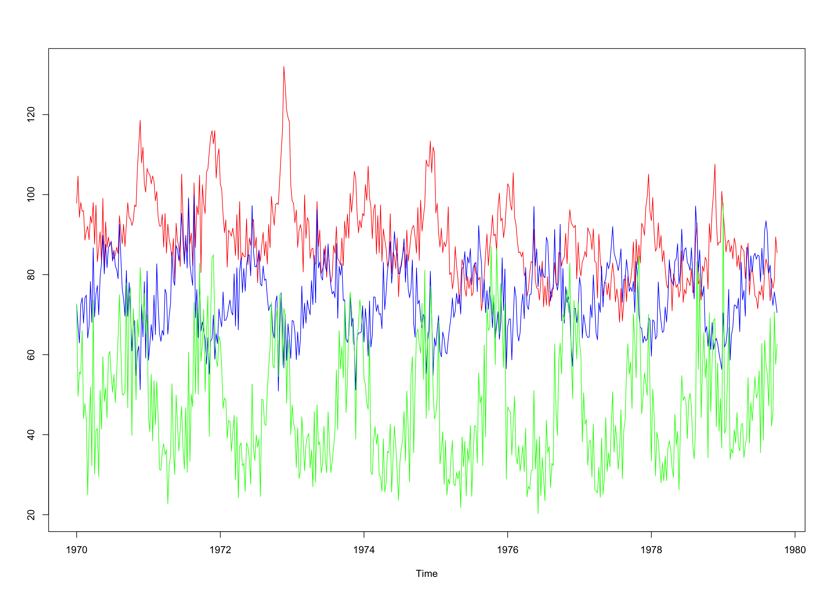
ts.plot(cmort, tempr, part, col = c("red", "blue", "green"))  # all on same plot (not shown) dev.new()

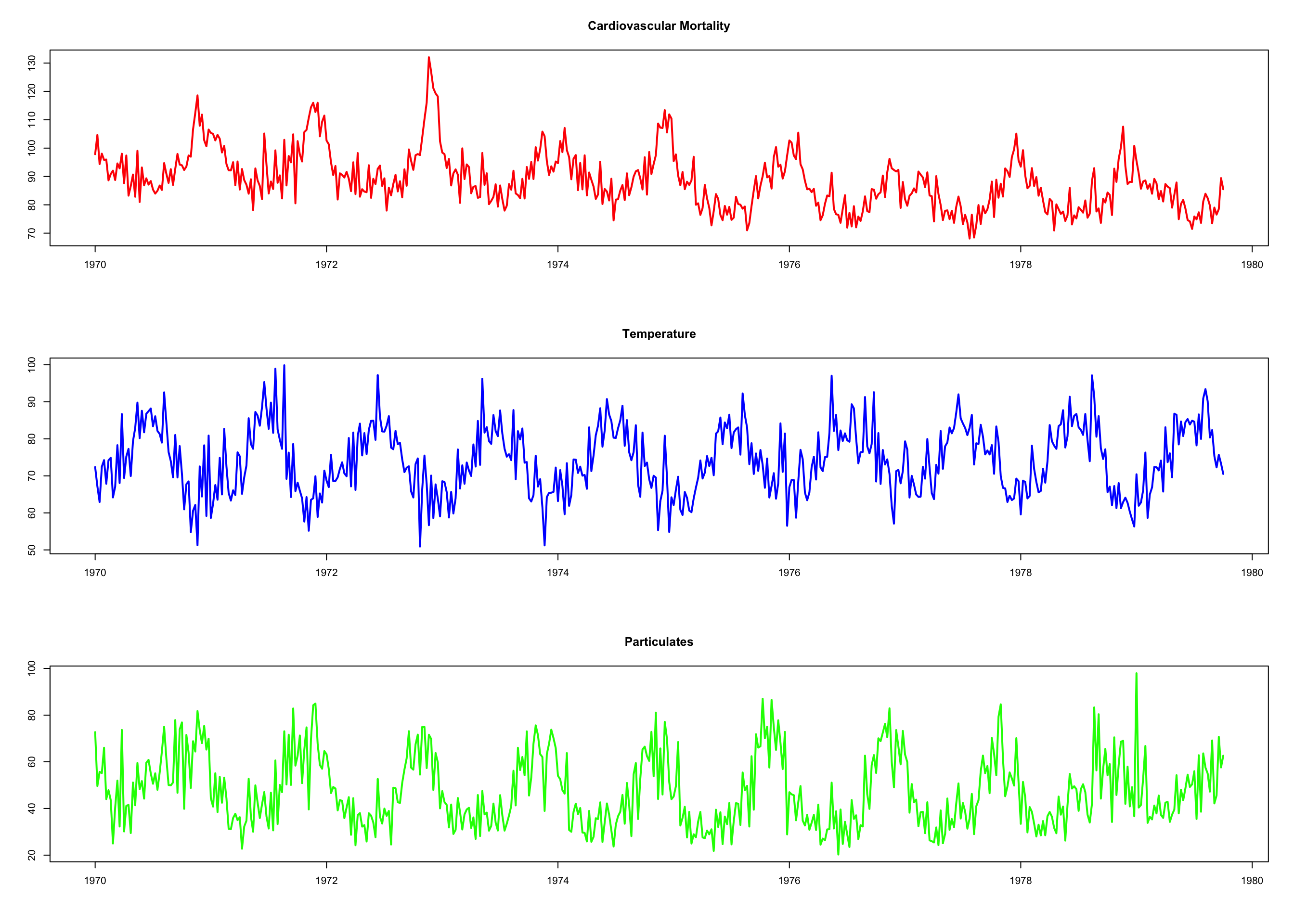
• Note:
  • We want to investigate the effects of temperature and pollution on weekly mortality in LA.
  • There are strong seasonal components in all series (winter/summer).
  • Downwards trend for cardiovascular mortality.
• We need more analysis to choose model candidates.

Here, scatterplots are informative (output on next slide):

pairs(cbind(Mortality = cmort, Temperature = tempr, Particulates = part))
temp <- tempr - mean(tempr)  # center temperature
temp2 <- temp^2
trend <- time(cmort)  # time

• There is possible linear relation between mortality and particulates
• Also, there is a curvilinear shape of temperature mortality curve: temperature extremes are associated with higher mortality

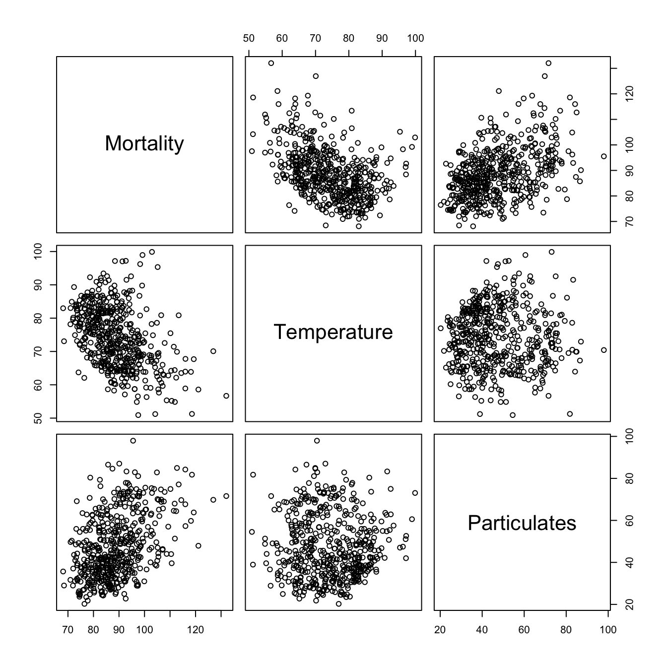
Based on the scatterplot matrix we consider the following models:

$$\begin{array}{rcl} M_t &=& \beta_0 + \beta_1 t + w_t \\ M_t &=& \beta_0 + \beta_1 t + \beta_2 (T_t-T_\cdot) +w_t \\ M_t &=& \beta_0 + \beta_1 t + \beta_2 (T_t-T_\cdot) +\beta_3(T_t-T_\cdot)^2+w_t \\ M_t &=& \beta_0 + \beta_1 t + \beta_2 (T_t-T_\cdot) +\beta_3(T_t-T_\cdot)^2+\beta_4 P_t+w_t \\ \end{array}$$

where \(T_\cdot=74.26\) is the temperature mean.

fit <- lm(cmort ~ trend + temp + temp2 + part, na.action = NULL)
summary(fit)  # regression results

...
## Residuals:
##      Min       1Q   Median       3Q      Max 
## -19.0760  -4.2153  -0.4878   3.7435  29.2448 
## 
## Coefficients:
##               Estimate Std. Error t value Pr(>|t|)    
## (Intercept)  2.831e+03  1.996e+02   14.19  < 2e-16 ***
## trend       -1.396e+00  1.010e-01  -13.82  < 2e-16 ***
## temp        -4.725e-01  3.162e-02  -14.94  < 2e-16 ***
## temp2        2.259e-02  2.827e-03    7.99 9.26e-15 ***
## part         2.554e-01  1.886e-02   13.54  < 2e-16 ***
## ---
## Signif. codes:  0 '***' 0.001 '**' 0.01 '*' 0.05 '.' 0.1 ' ' 1
## 
## Residual standard error: 6.385 on 503 degrees of freedom
## Multiple R-squared:  0.5954,	Adjusted R-squared:  0.5922 
...

summary(aov(fit))  #ANOVA table (compare to next code chunk!)

##              Df Sum Sq Mean Sq F value Pr(>F)    
## trend         1  10667   10667  261.62 <2e-16 ***
## temp          1   8607    8607  211.09 <2e-16 ***
## temp2         1   3429    3429   84.09 <2e-16 ***
## part          1   7476    7476  183.36 <2e-16 ***
## Residuals   503  20508      41                   
## ---
## Signif. codes:  0 '***' 0.001 '**' 0.01 '*' 0.05 '.' 0.1 ' ' 1

\(\rightarrow\) Each addition is significant.

summary(aov(lm(cmort ~ cbind(trend, temp, temp2, part))))  # Table 2.1

##                                  Df Sum Sq Mean Sq F value Pr(>F)    
## cbind(trend, temp, temp2, part)   4  30178    7545     185 <2e-16 ***
## Residuals                       503  20508      41                   
## ---
## Signif. codes:  0 '***' 0.001 '**' 0.01 '*' 0.05 '.' 0.1 ' ' 1

num <- length(cmort)  # sample size
AIC(fit)/num - log(2 * pi)  # AIC

## [1] 4.721732

BIC(fit)/num - log(2 * pi)  # BIC

## [1] 4.771699

AICc <- log(sum(resid(fit)^2)/num) + (num + 5)/(num - 5 - 2)  # AICc
AICc

## [1] 4.722062

Example: Regression with lagged variables #

Recall the SOI and (fish) Recruitment series: previous data analysis suggested that SOI led Recruitment by six months. The relationship is not linear, but we consider (for now) $$R_t=\beta_0+\beta_1 S_{t-6} + w_t,$$ which becomes, after fitting (if \(w_t\) is assumed Gaussian white) $$R_t=65.79-44.28_{(2.78)} S_{t-6},$$ with \(\hat{\sigma}_w=22.5\) (on 445 degrees of freedom):

fish <- ts.intersect(rec, soiL6 = stats::lag(soi, -6), dframe = TRUE)
summary(fit1 <- lm(rec ~ soiL6, data = fish, na.action = NULL))
...
##             Estimate Std. Error t value Pr(>|t|)    
## (Intercept)   65.790      1.088   60.47   <2e-16 ***
## soiL6        -44.283      2.781  -15.92   <2e-16 ***
...

\(\rightarrow\) SOI is a strong predictor of Recruitment

Exploratory Data Analysis (TS 2.2) #

Context #

Remember $$x_t = \mu_t +y_t$$ is called trend stationary if \(y_t\) is stationary.

“Removing” \(\mu_t\) is called “detrending”, and we distinguish two types thereof:

• via regression: This involves fitting a regression model for \(\hat{\mu}_t\) (as per the previous section).
  • This is a parametric approach: \(\hat{\mu}_t\) is known, but for parameter and model risk.
• via differencing: This involves modifying the series by looking at differences over time, rather than absolute values.
  • This is a non parametric approach: we do not need to specify a model, but \(\hat{\mu}_t\) remains unknown and unmodelled.

Detrending via regression #

Example: Chicken prices detrended via regression #

From before:

fit <- lm(chicken ~ time(chicken), na.action = NULL)  # regress chicken on time
plot(resid(fit), type = "l", main = "Price of chicken detrended via regression
     (spot price, Georgia docks, 08/01-07/16)")

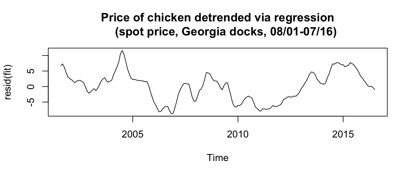
• Note that the residuals are, by definition, equal to \(\hat{y}_t\) which we would like to be stationary.
• Here we have \(\mu_t=\beta_0+\beta_1 t\) as before

Differencing #

What if \(\mu_t\) does not look like a linear trend?

• In that case detrending via (linear) regression is not adequate
• This may suggest that the trend / mean is random

In this case one can look at the difference from one point to the next: $$\nabla x_t \equiv x_t-x_{t-1}$$ If the mean is random, this should yield the difference in random means (from \(t-1\) to \(t\)), plus the difference of the detrended (assumed stationary) underlying series (which we are seeking).

As an example, consider the simplest model with a random mean: the random walk with drift $$\mu_t=\delta+\mu_{t-1}+w_t,$$ where \(w_t\) is the random component of the mean.

Using differencing yields $$\nabla x_t \equiv x_t-x_{t-1}=(\mu_t+y_t)-(\mu_{t-1}+y_{t-1})=\delta+w_t+(y_t-y_{t-1}),$$ where \(z_t = y_t-y_{t-1}\) is stationary, and hence \(x_t-x_{t-1}\) is stationary too.

Note:

• a first difference removes a linear (random) trend
• a second difference ( \(\nabla^2\), differencing the differenced series) removes a quadratic trend
• etc…

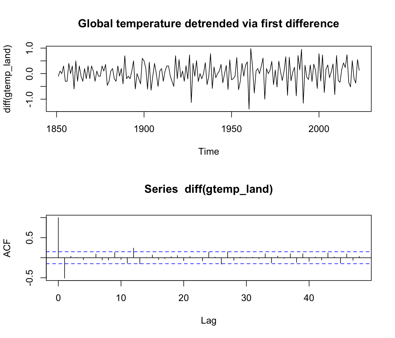
Example: Differencing Global Temperatures #

Remember the Global Temperatures series:

plot(gtemp_land, type = "o", ylab = "Global Temperature Deviations",
  main = "Yearly average global temperature deviations (1880-2015) in degrees centigrade (base period: 1951-1980)")

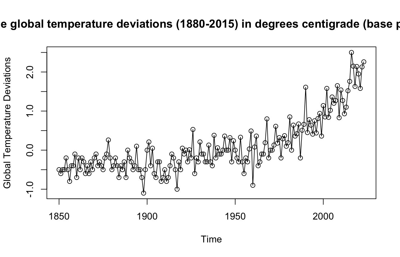
mean(diff(gtemp_land))=0.0159538

par(mfrow = c(2, 1))
plot(diff(gtemp_land), type = "l", main = "Global temperature detrended via first difference")
acf(diff(gtemp_land), 48)

How does differencing compare with regression? #

• Differencing can be seen as “without loss of generality” as compared to the regression case.
• If the regression model was appropriate, we would have $$\mu_t=\beta_0+\beta_1 t$$ and differencing would lead to $$\nabla x_t=x_t-x_{t-1}=(\mu_t+y_t)-(\mu_{t-1}+y_{t-1})=\beta_1+y_t-y_{t-1},$$ which is stationary (residuals \(y_t\) are uncorrelated normal in a regression).

Example: Chicken prices detrended via differencing #

plot(diff(chicken), type = "l", main = "Price of chicken detrended via first difference
     (spot price, Georgia docks, 08/01-07/16)")

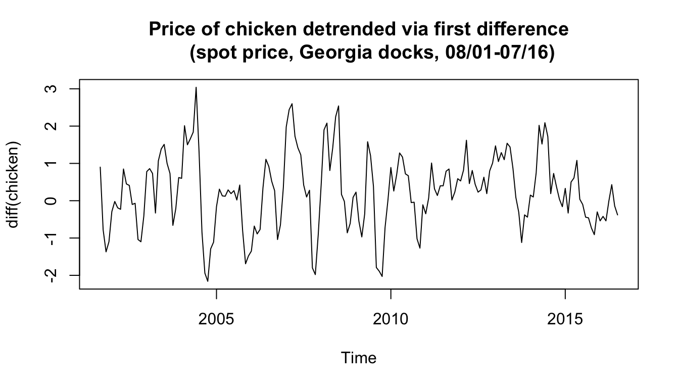
• Although results are different, both methods can potentially work.
• The question is whether the drift is likely deterministic or random. If random, differencing could remove it without making
  an assumption about it.

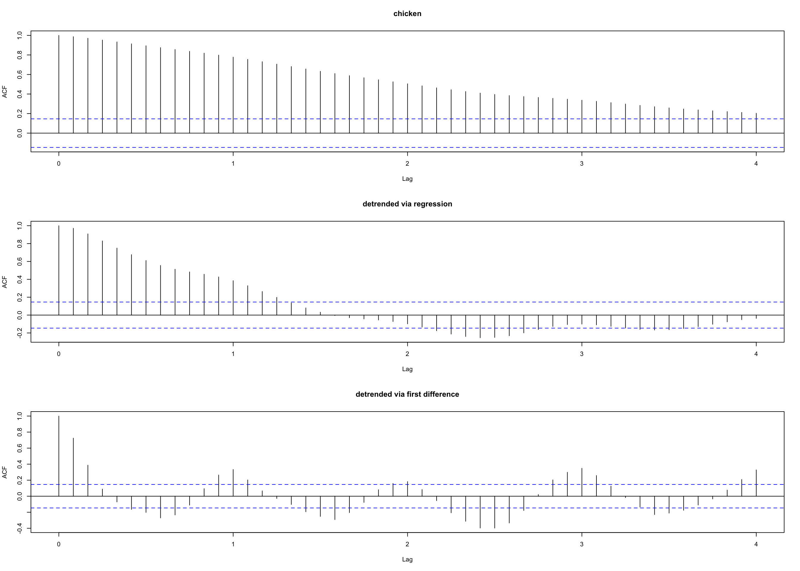
Comparison of autocorrelation in the residuals #

par(mfrow = c(3, 1))  # plot ACFs
acf(chicken, 48, main = "chicken")
acf(resid(fit), 48, main = "detrended via regression")
acf(diff(chicken), 48, main = "detrended via first difference")

See next slide for those graphs:

• The ACF of residuals after differencing exhibits an annual cycle that was obscured in the regressed data.

That was probably due to the (erroneous) assumption of \(w_t\) (the errors in the regression) to be white.

Backshift operator #

We define the backshift operator by $$Bx_t = x_{t-1}$$ and extend it to powers \(B^2x_t = B(Bx_t) = Bx_{t-1} = x_{t-2},\) and so on. Thus, $$B^kx_t =x_{t-k}.$$ Note:

• This notation allows for compact definition of models, and easier algebraic calculations.
• The forward-shift operator is the inverse such that $$x_t=B^{-1}Bx_t=B^{-1}x_{t-1}.$$
• We define differences of order \(d\) as $$\nabla^d=(1-B)^d.$$

Transformations #

• Obvious aberrations and nonlinear behaviour, if present, can lead to nonstationarity.
• Transformations may be useful to equalise the variability over the length of a single series. A particularly useful transformation is $$y_t = \log x_t,$$ which tends to suppress larger fluctuations that occur over portions of the series where the underlying values are larger.
  (Think, for instance, of the Johnson & Johnson data)
• Transformations can also be used to improve the approximation to normality or to improve linearity in predicting the value of one series from another.

Scatterplot matrices #

• This is another preliminary data processing technique, to visualise the relations between series at different lags.
• The ACF—a single number—focuses on linear predictability only (since it displays correlations).
• Scatterplots (one for each lag) are informative to diagnose nonlinear relationships: they display the whole profile of the relation.
• They give a visual sense of which lag will lead to the best predictability
• This can be done for a single series or between two series—say, \(y_t\) vs \(x_{t-h}\)
• The red lines are locally weighted “scatterplot smoothing lines” (more precisely, lowess lines—see next section); they help identify non-linear relationships.

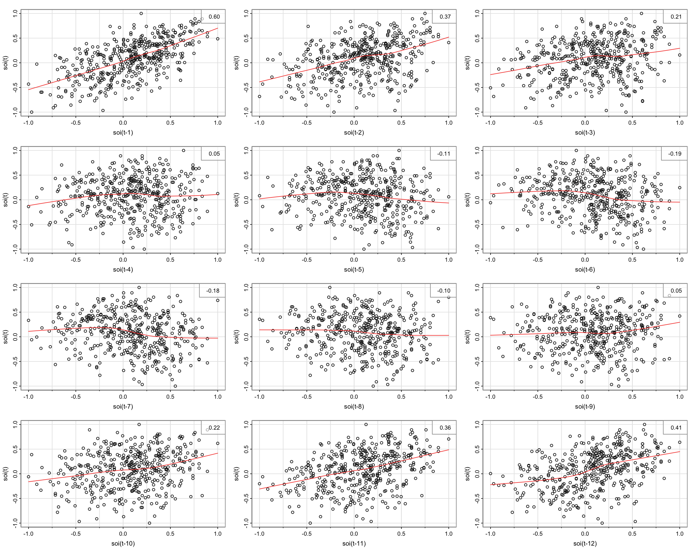
Example: SOI vs recruitment #

Scatterplot for SOI only (next slide)

lag1.plot(soi, 12)

• The red lines are more or less linear for lagged SOI \(\rightarrow\) sample autocorrelations are meaningful

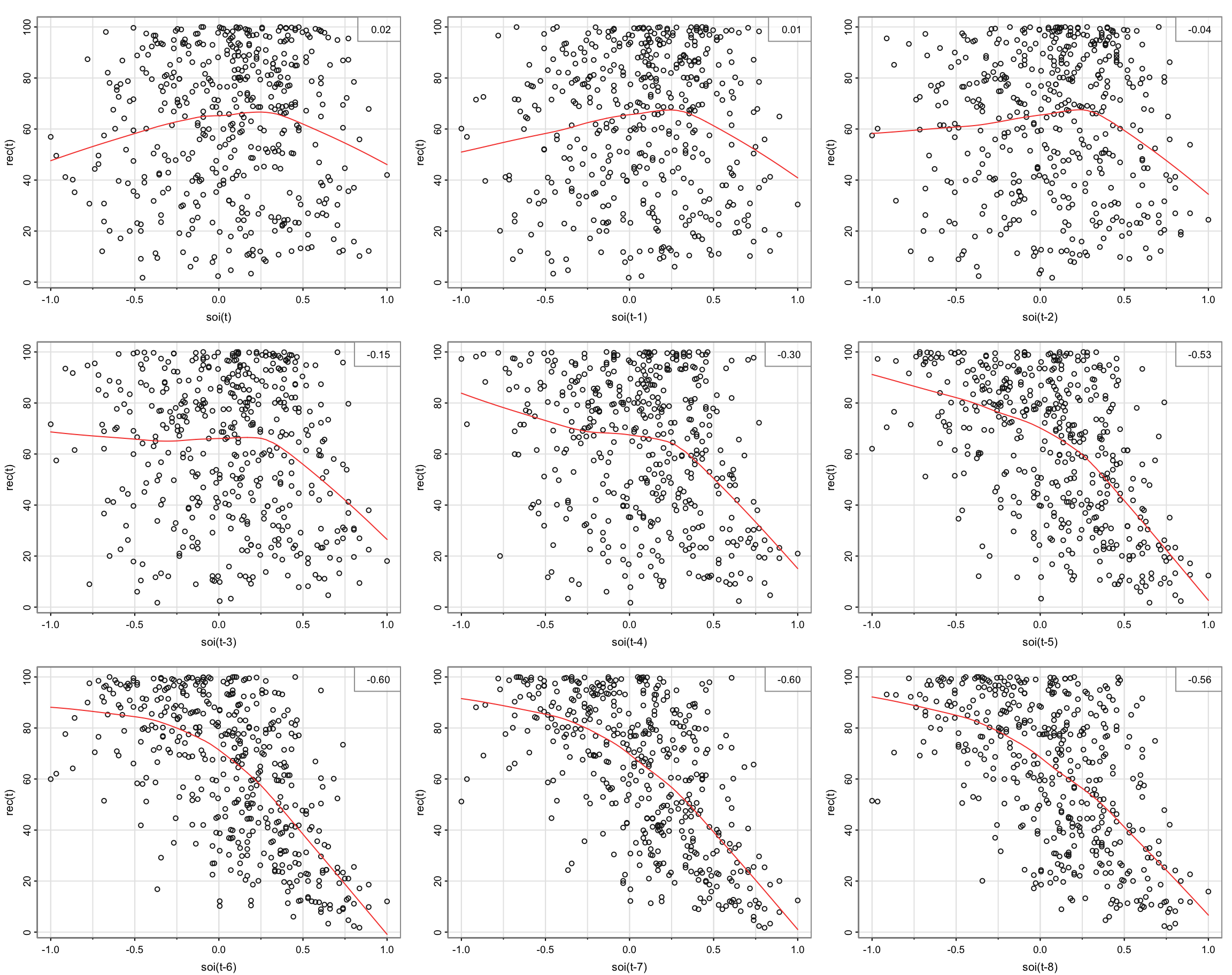
Scatterplot for Recruitment \(R_t\) vs SOI \(h\) lags earlier \(S_{t-h}\) (following slide)

lag2.plot(soi, rec, 8)

• Red lines are highly nonlinear around lag 6. However, they seem to be linear for given sign of SOI

How would you model this nonlinear relationship?

Using dummy variables we can model this:

$$\begin{array}{rcl} R_t &=& \beta_0+\beta_1S_{t-6}+\beta_2D_{t-6}+\beta_3D_{t-6}S_{t-6}+w_t \\ &=& \left\{ \begin{array}{ll} \beta_0+\beta_1 S_{t-6}+w_t & \text{ if }S_{t-6}<0, \\ (\beta_0\alert{+\beta_2})+(\beta_1\alert{+\beta_3}) S_{t-6}+w_t & \text{ if }S_{t-6}\alert{\ge}0, \end{array} \right. \end{array}$$ where \(D_t=0\) if \(S<0\) (1 otherwise).

dummy <- ifelse(soi < 0, 0, 1)  # for the piecewise regression
fish <- ts.intersect(rec, soiL6 = stats::lag(soi, -6), dL6 = stats::lag(dummy,
  -6), dframe = TRUE)
summary(fit <- lm(rec ~ soiL6 * dL6, data = fish, na.action = NULL))

...
##             Estimate Std. Error t value Pr(>|t|)    
## (Intercept)   74.479      2.865  25.998  < 2e-16 ***
## soiL6        -15.358      7.401  -2.075   0.0386 *  
## dL6           -1.139      3.711  -0.307   0.7590    
## soiL6:dL6    -51.244      9.523  -5.381  1.2e-07 ***
...

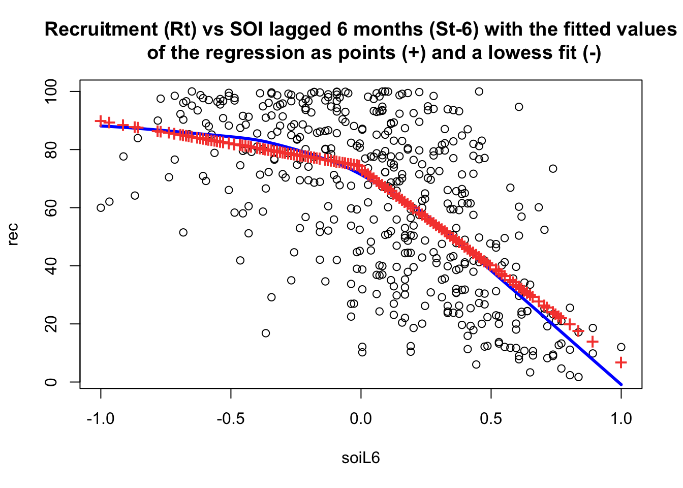
attach(fish)

plot(soiL6, rec, main = "Recruitment (Rt) vs SOI lagged 6 months (St-6) with the fitted values
     of the regression as points (+) and a lowess fit (-)")
lines(lowess(soiL6, rec), col = "blue", lwd = 3)
points(soiL6, fitted(fit), pch = "+", col = 2, cex = 1.5)

plot(resid(fit), main = "Residuals of recruitment (Rt) vs SOI lagged 6 months (St-6)
     with the fitted values of the regression as points (+) and a lowess fit (-)")

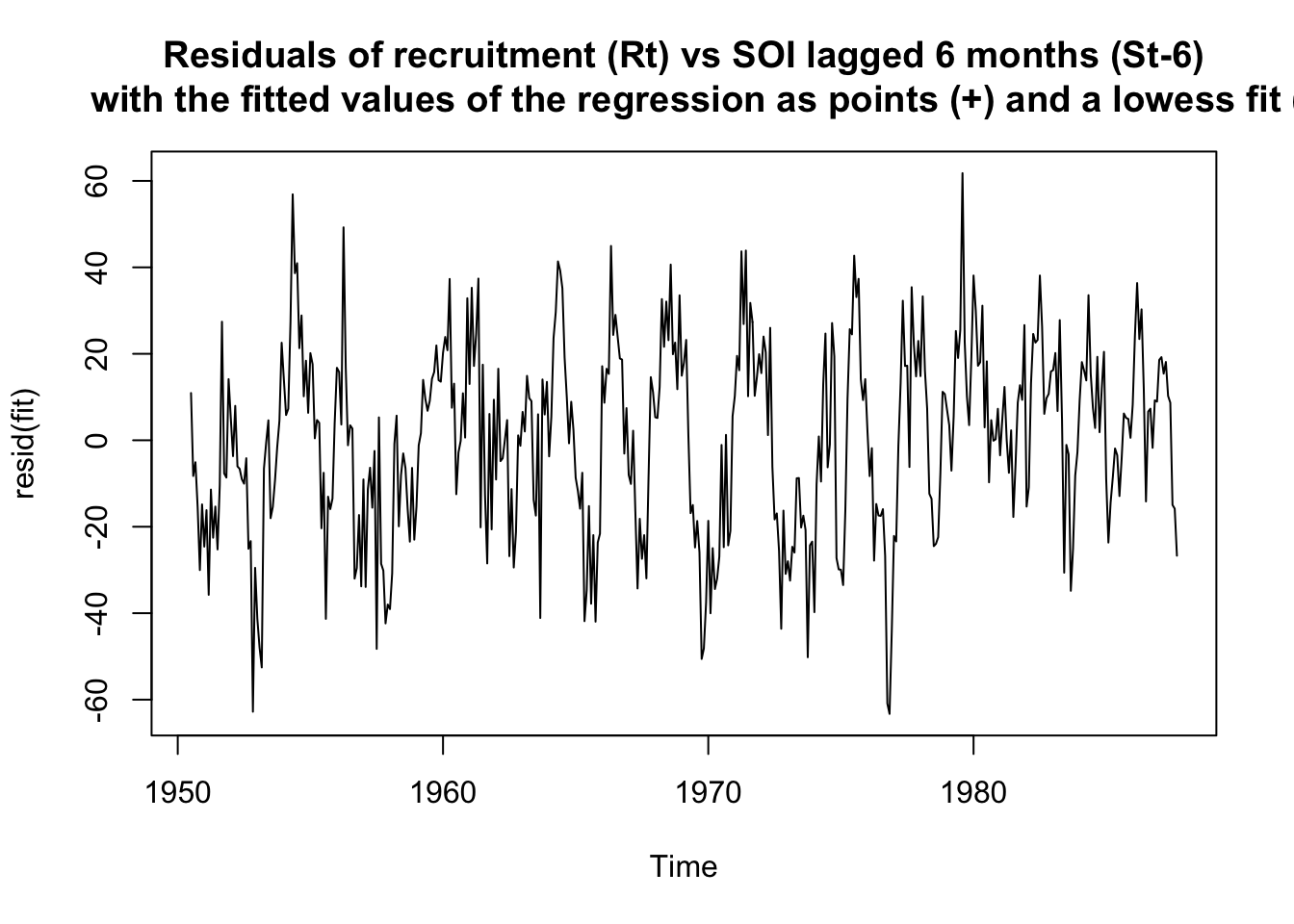
acf(resid(fit), main = "ACF of the residuals")  # obviously not noise

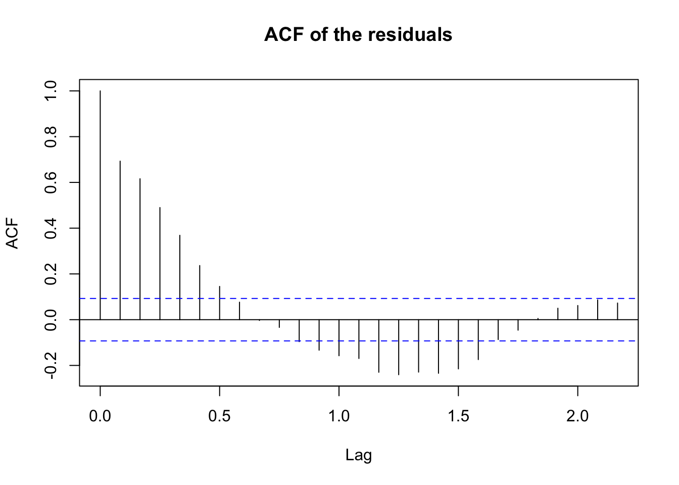
• residuals are not white noise - we would need to model cycles next

Smoothing in the Time Series Context (TS 2.3) #

Introduction #

• The first difference \(\nabla\) is an example of linear filter applied to eliminate a trend.
• Other filters, formed by averaging values near \(x_t\), can produce adjusted series that eliminate other kinds of unwanted fluctuations.
• This can help discover certain traits in a time series, such as long-term trend and seasonal components.
• Here we review such filtering techniques, with illustrations.

Example: SOI #

ts.plot(soi, ylab = "", xlab = "", main = "South Oscillation Index SOI
        (changes in air pressure, related to sea surface temperatures, in the central Pacific Ocean)")

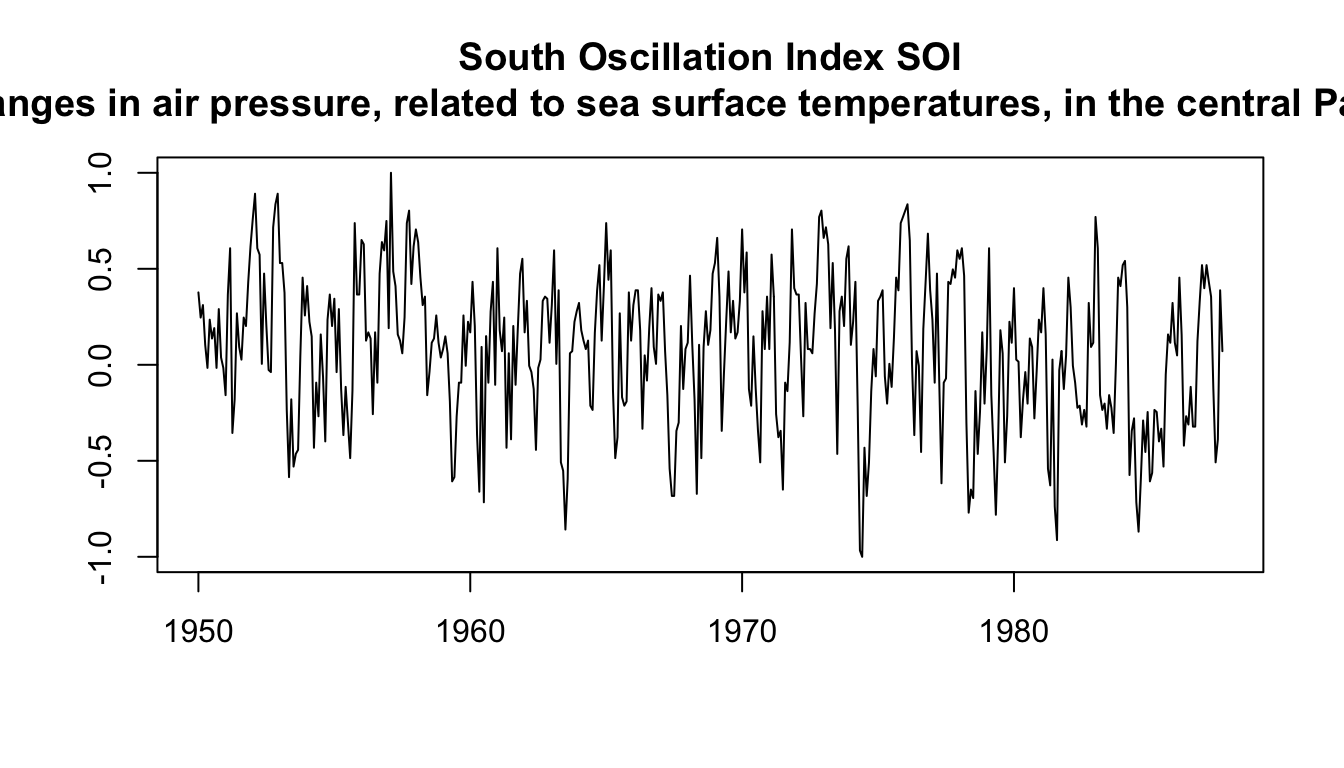
How easy is it to see the El Niño cycles, and distinguish them from the (strong) annual cycles?

Moving Average Smoother #

If \(x_t\) represents the observations, then $$m_t=\sum_{j=-k}^k a_j x_j,$$ where $$a_j=a_{-j}\ge 0,\quad\text{ and where }\quad \sum_{j=-k}^k a_j=1,$$ is a symmetric (two-sided) moving average of the data.

Note:

• When their profile is flat, the weights \(a_j\) are sometimes referred to as “boxcar-type” weights.

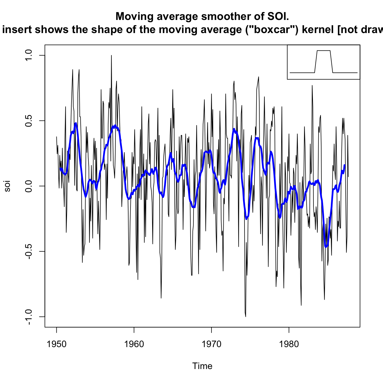
Example: Moving Average Smoother on SOI #

wgts <- c(0.5, rep(1, 11), 0.5)/12
soif <- stats::filter(soi, sides = 2, filter = wgts)
par()
plot(soi, main = "Moving average smoother of SOI.
     The insert shows the shape of the moving average (\"boxcar\") kernel [not drawn to scale]")
lines(soif, lwd = 3, col = "blue")
par(fig = c(0.65, 1, 0.65, 1), mar = c(5, 3.5, 4.1, 2.1), new = TRUE)  # the insert
nwgts <- c(rep(0, 20), wgts, rep(0, 20))
plot(nwgts, type = "l", ylim = c(-0.02, 0.1), xaxt = "n", yaxt = "n",
  ann = FALSE)

• This particular method removes (filters out) the obvious annual temperature cycles, and helps emphasize the El Niño cycles
• However, it is still quite choppy, probably due to the (relatively non smooth) boxcar weights

Kernel Smoothing #

If \(x_t\) represents the observations, then $$m_t=\sum_{i=1}^n w_i(t) x_i,\text{ where } w_i(t)=\frac{K\left(\frac{t-i}{b}\right)}{\sum_{k=1}^n K\left(\frac{t-k}{b}\right)}$$ are the weights, and where \(K(\cdot)\) is a kernel function.

• Each \(m_t\) uses all the \(x_t\)’s, contrary to the moving average smoother
• A typical kernel is the normal kernel, $$K(z)=\frac{1}{\sqrt{2\pi}}e^{-\frac{1}{2}z^2}.$$

In R, the function to use is ksmooth(x, y, kernel = c("box", "normal"), bandwidth) Note:

• The wider the bandwidth, the smoother the result
• Kernels are scaled such that the kernel quartiles (viewed as probability densities) are at \(\pm 0.25\times\)``bandwidth
  • E.g., for the normal distribution, the quartiles are \(\pm 0.674\)—this means \(\Phi(0.674)-0.5=25\%\)

In the next example, the bandwidth is 1 to correspond to approximately smoothing a little over one year:

• The standard normal quartile 0.674 is scaled to be at \(0.25\times 1=0.25\), so \(\pm 0.25\) after scaling corresponds to 50% of the original standard normal
• \(\pm 0.5\) thus corresponds to \(\pm 2\cdot 0.674=\pm 1.328\) in terms of original standard normal, which corresponds to \(2\times \left[\Phi(1.328)-0.5\right]\approx 82.2\%\) of the density.
• Similarly, \(\pm 0.75\) corresponds to \(\approx 95.6\%\) of the density.

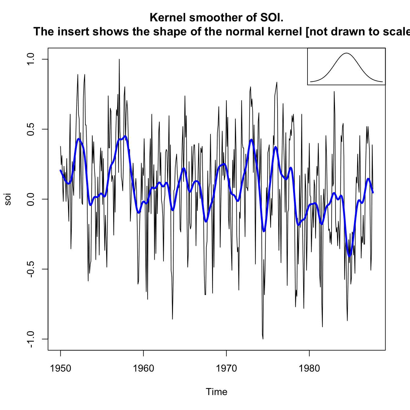
Example: Kernel smoothing on SOI #

plot(soi, main = "Kernel smoother of SOI.
     The insert shows the shape of the normal kernel [not drawn to scale]")
lines(ksmooth(time(soi), soi, "normal", bandwidth = 1), lwd = 3,
  col = "blue")
par(fig = c(0.65, 1, 0.65, 1), mar = c(5, 3.5, 4.1, 2.1), new = TRUE)  # the insert
gauss <- function(x) {
  1/sqrt(2 * pi) * exp(-(x^2)/2)
}
x <- seq(from = -3, to = 3, by = 0.001)
plot(x, gauss(x), type = "l", ylim = c(-0.02, 0.45), xaxt = "n",
  yaxt = "n", ann = FALSE)

Lowess #

• Lowess is complex, but close to the idea of \(k\)-nearest neighbor regression, where one uses only the data $$(x_{t-k/2},\ldots,x_t,\ldots,x_{t+k/2})$$ to predict \(x_t\) via regression, and then sets \(m_t=\hat{x}_t\).
• In R, the function is lowess(x,f=2/3) where f is the smoother span with default value \(2/3\)
• The smoother span is the proportion of points in the plot which influence the smooth at each value. Larger values give more smoothness.
• One can also smooth a time series x as function of another series y. We use then lowess(x,y).

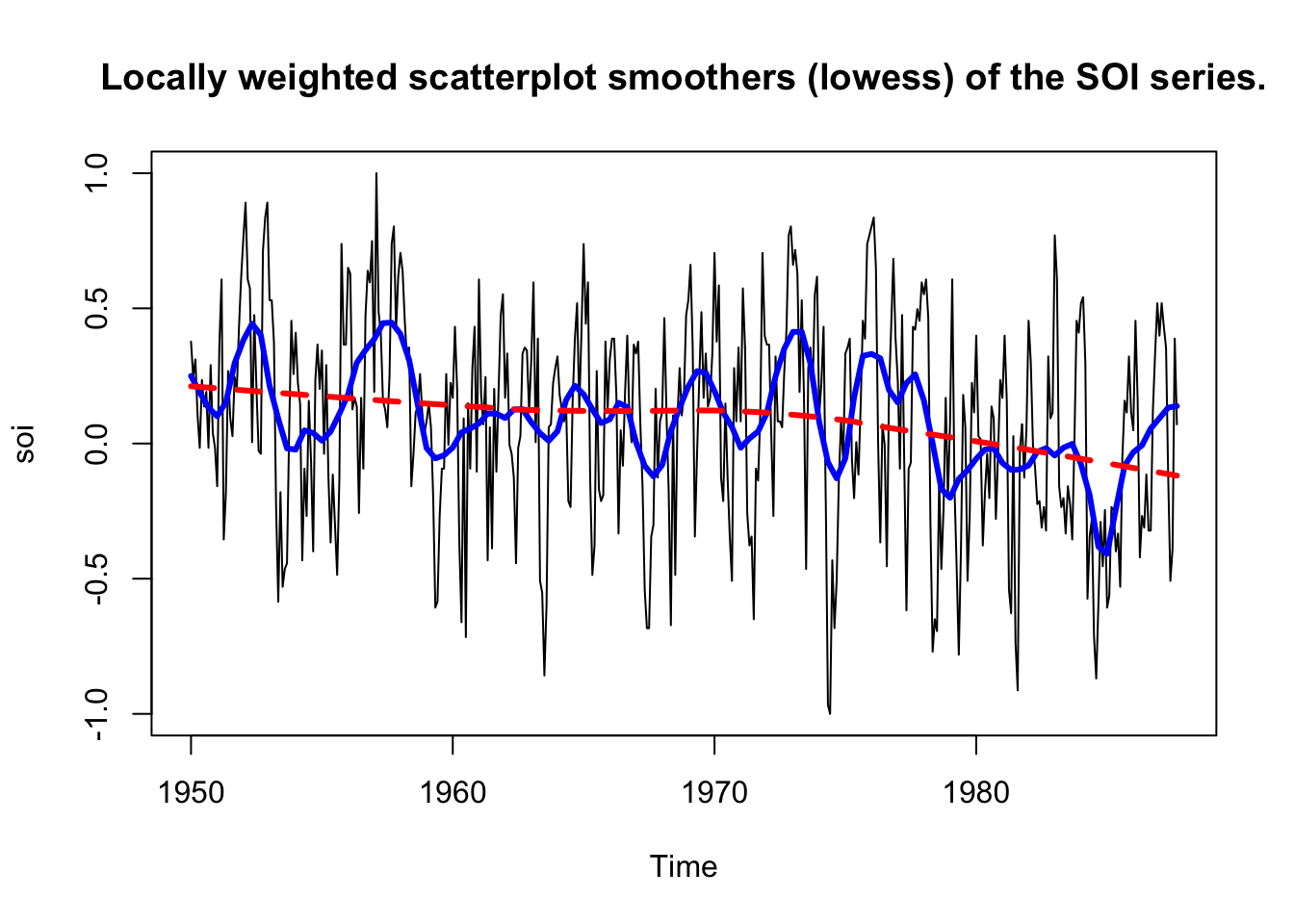
Example: Lowess on SOI #

plot(soi, main = "Locally weighted scatterplot smoothers (lowess) of the SOI series.")
lines(lowess(soi, f = 0.05), lwd = 3, col = "blue")  # El Nino cycle
lines(lowess(soi), lty = 2, lwd = 3, col = "red")  # trend (with default span)

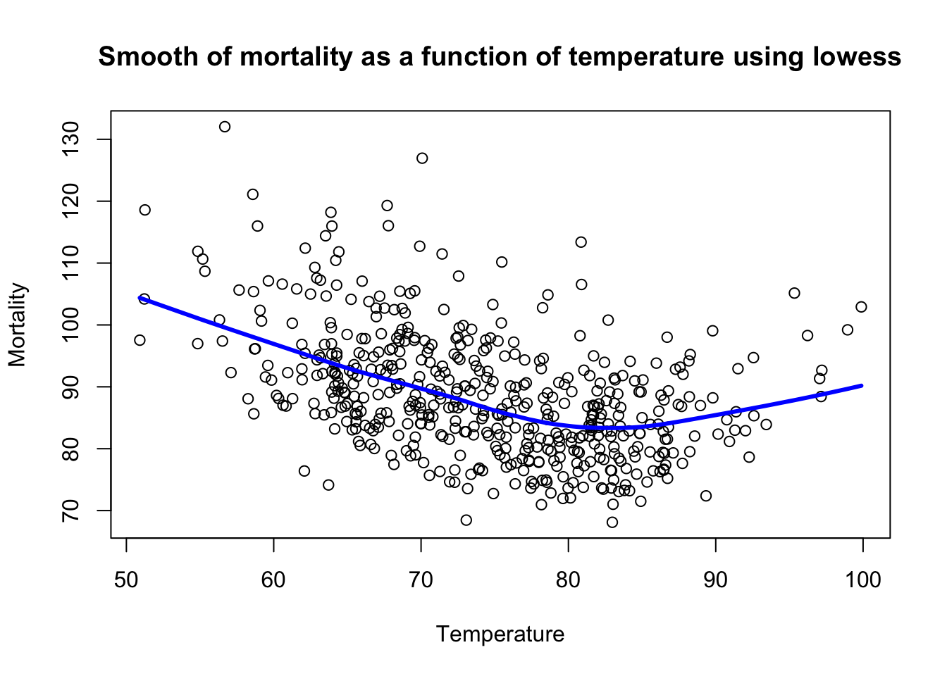
Example: Lowess of mortality as a function of temperature #

plot(tempr, cmort, xlab = "Temperature", ylab = "Mortality",
  main = "Smooth of mortality as a function of temperature using lowess")
lines(lowess(tempr, cmort), lwd = 3, col = "blue")

Smoothing splines #

Preliminary: Polynomial regression #

A polynomial regression in terms of time would involve setting $$x_t=m_t+w_t,\text{ where }m_t=\beta_0+\beta_1 t+\beta_2 t^2 + \beta_3 t^3 + \ldots.$$ Then, \(m_t\) would be fit to data using ordinary least squares (which assumes \(w_t\) is normal).

One possible extension is to fit polynomials to the series in a piecewise fashion:

• Divide time into $k$ intervals $$[t_0=1,t_1],[t_{1+1},t_2],\ldots,[t_{k-1}+1,t_k=n],$$ where **$t_0, t_1, \ldots, t_k$ are called **.
• Then, in each interval, one fits a polynomial regression, typically of order 3 (in which case these are called splines).

Smoothing splines #

Here we minimise a compromise between fit and smoothness: $$\sum_{t=1}^n [x_t-m_t]^2+\lambda \int \left(m_t''\right)^2 dt,$$ where \(m_t\) is a cubic spline with a knot at each \(t\). The degree of smoothness is controlled by \(\lambda\), and is an extra parameter that is useful.

• if \(\lambda=0\) then \(m_t=x_t\) which is useless and smoothes nothing.
• if \(\lambda=\infty\) we are infinitely focussed on the second derivative of \(m_t\), so that \(m_t=c+vt\) which is extremely smooth.
• \(\lambda\) allows thus for a spectrum between linear regression \((\infty)\) and the data \((0)\) —the larger the \(\lambda\), the smoother the fit.

The fact that one does not need to choose knots can be seen as an advantage (objective), but this is why ” \(\lambda\) smoothness” is required
to avoid overfitting.

Example: Splines on SOI #

plot(soi, main = "Smoothing splines fit to the SOI series
     (spar=0.5 in blue to emphasise El Niño cycle, and spar=1 in red to emphasise the trend)")
lines(smooth.spline(time(soi), soi, spar = 0.5), lwd = 3, col = "blue")
lines(smooth.spline(time(soi), soi, spar = 1), lty = 2, lwd = 3,
  col = "red")

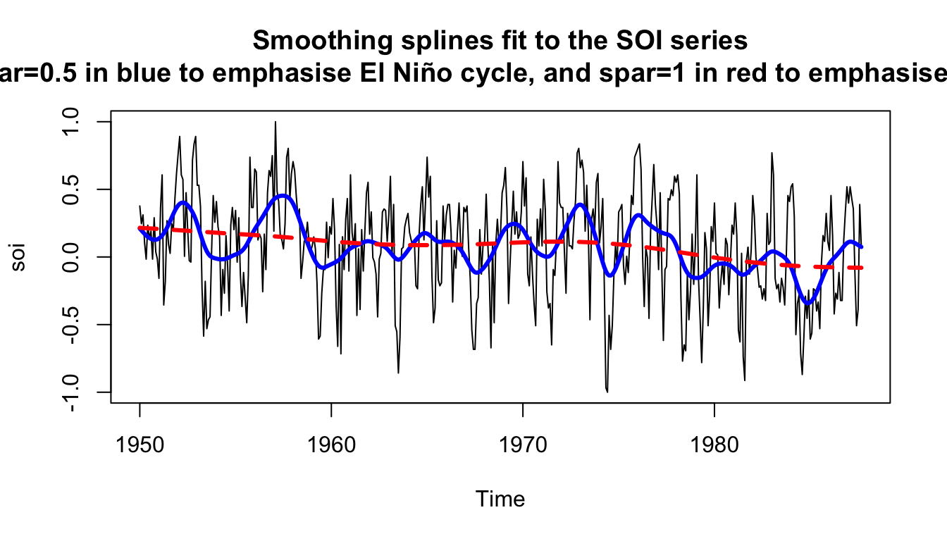
The parameter spar is monotonically related to \(\lambda\).

References #