Introduction (TS 1.0) #

Definition #

• Consider data of the same nature that have been observed at different points in time
• The mere fact that they are of the same nature means that they are likely related in one way or another - let’s call those `correlations’
  (an acceptable term in this context as we focus on this measure, at least in this course)
• This is in contrast with the usual “i.i.d.” assumptions associated with a sample of outcomes of a random variable
• This invalidates some of the techniques we know, and brings additional difficulties, but also opportunities! (such as forecasting)

Definition: “The systematic approach by which one goes about answering the mathematical and statistical questions posed by these time correlations is commonly referred to as time series analysis.”

Applications #

The applications of time series are many, and crucial in many cases:

• Economics: unemployment, GDP, CPI, etc $\dots$
• Finance: share prices, indices, etc $\dots$
• Medicine: COVID-19 cases and fatalities, biometric data for a patient (blood pressure, iron levels, $\dots$ ), etc $\dots$
• Global warming: ocean temperatures, ${\text{CO}}_2$ levels, concentration of particulates in the atmosphere, sea levels, all in relation with another, and with many others
• Actuarial studies: frequency and severity of claims in a LoB, mortality (at different ages, in different locations, $\dots$), superimposed inflation, IBNR claims, etc $\dots$

Process for time series analysis #

Sketch of process:

• Careful examination of data plotted over time (Module 7)
• Compute major statistical indicators (Modules 7 and 8)
• Guess an appropriate method/model for analysing the data (Modules 8 and 9)
• Fit and assess your model (Module 9)
• Use your model to perform forecasts if relevant (Module 10)

We distinguish two types of approaches:

• Time domain approach: investigate lagged relationships (impact of today on tomorrow)
• Frequency domain approach: investigate cycles (understand regular variations)

In actuarial studies, both are relevant.

Examples (TS 1.1) #

Johnson & Johnson quarterly earnings per share #

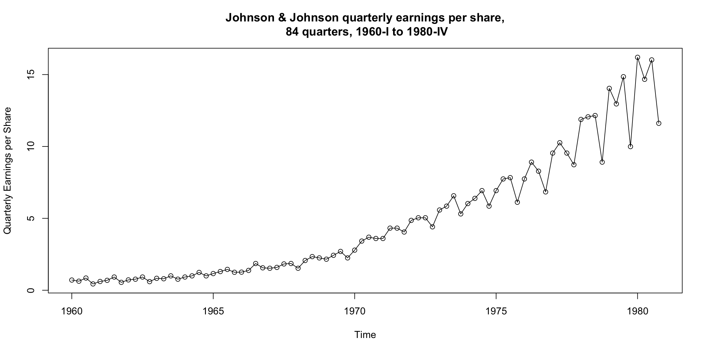
What is the primary pattern?
Can you see any cyclical pattern as well?
How does volatility change over time (if at all)?

Global mean land-ocean temperature index #

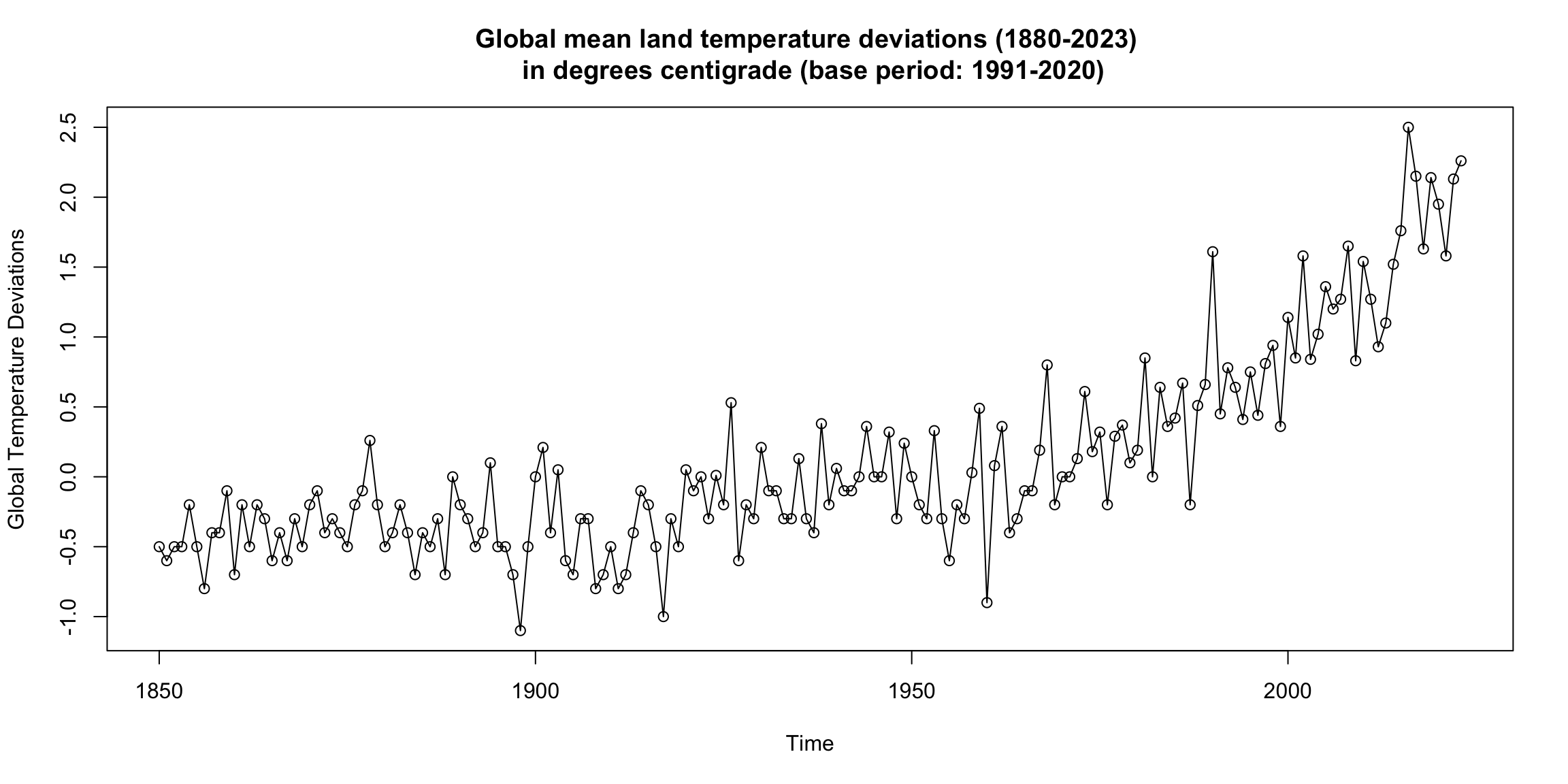
Can you see a trend? Are there periods of continuous increase?
What would be the main focus for global warming: trend or cycles?

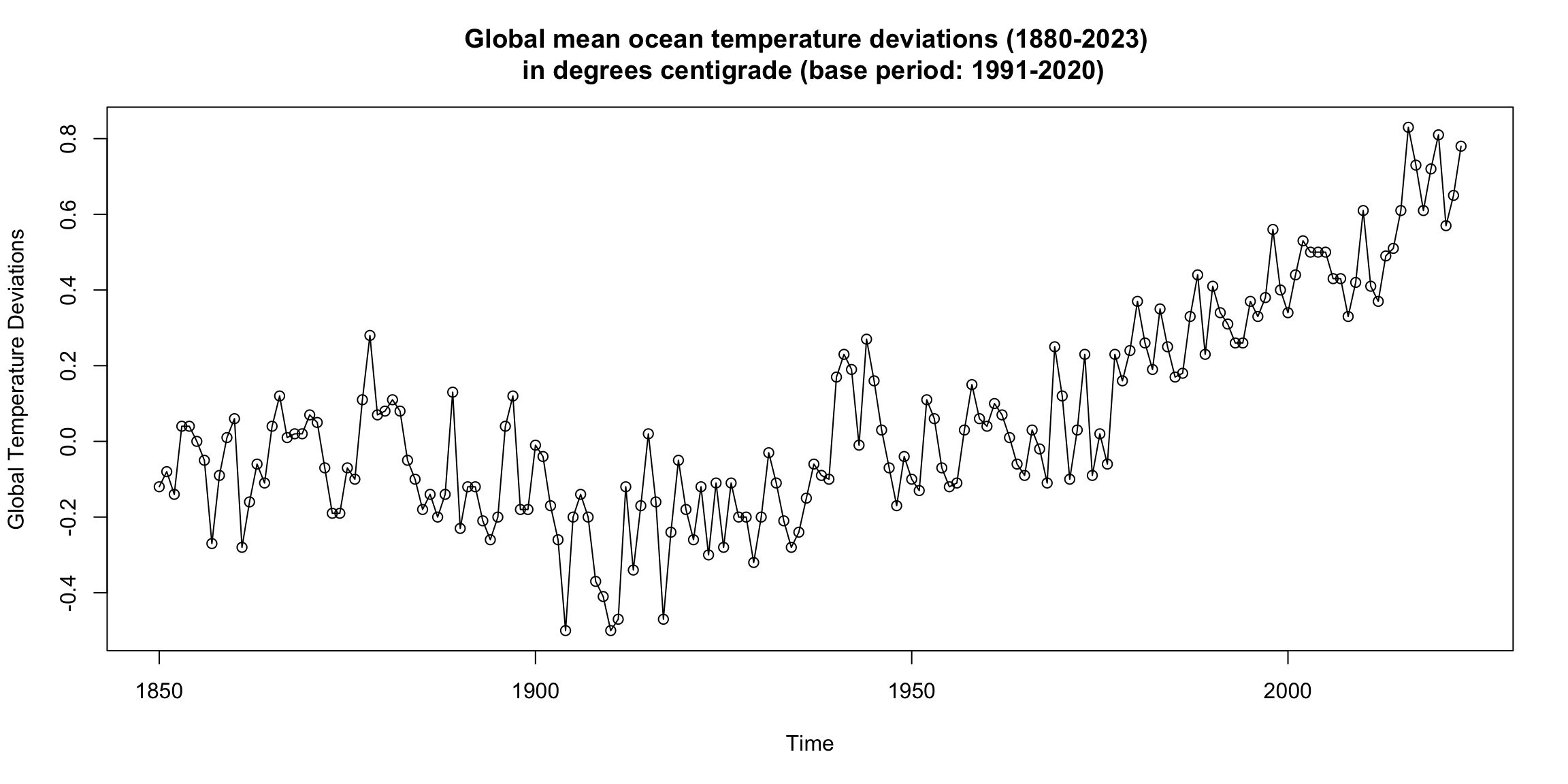
How do these graphs support the global warming thesis?

Dow Jones Industrial Average #

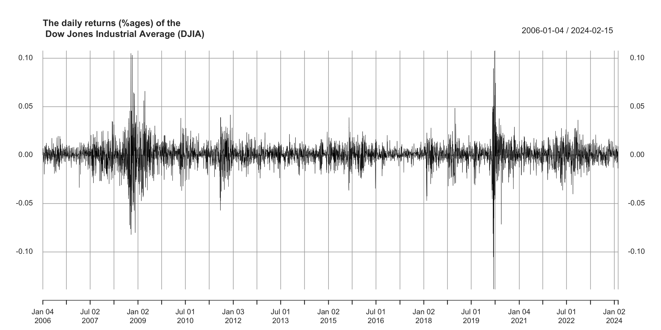
How is this time series special?
What qualities would a good forecast model need to have?

Analysis of two series together: El Niño & fish population #

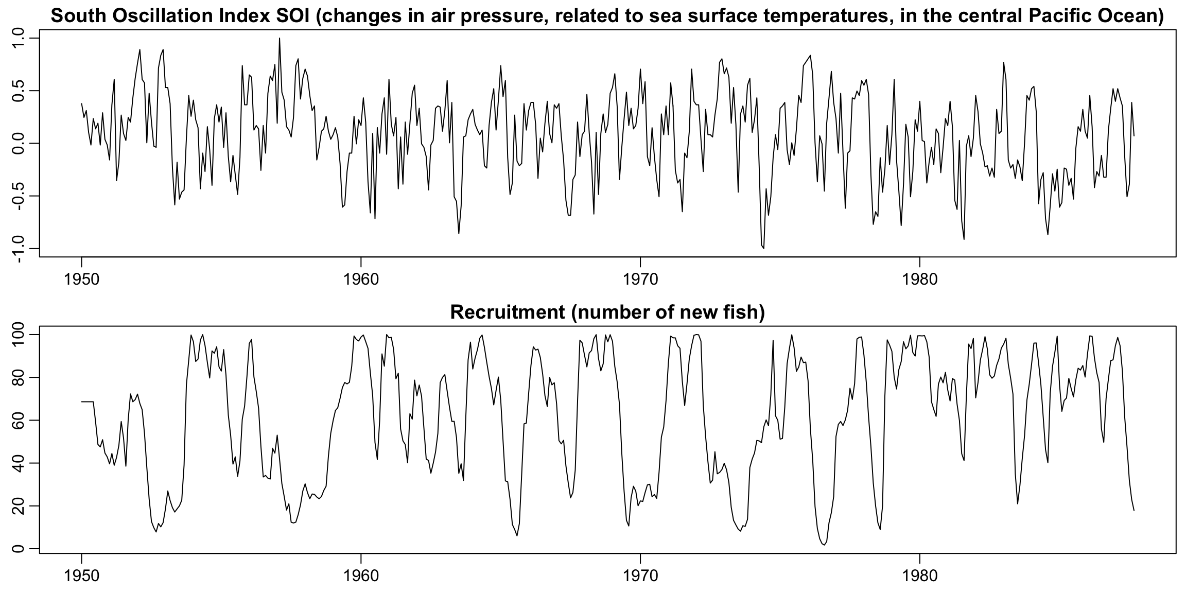
How many cycles can you spot?
Is there a relationship between both series?

Signals within noise #

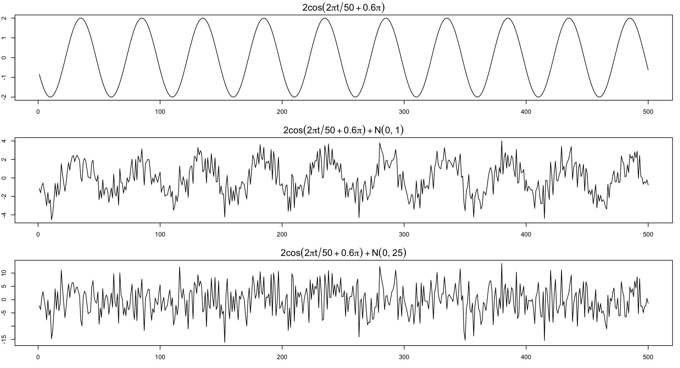
Typically we only see the the signal obscured by noise.

Basic models (TS 1.2) #

Preliminaries #

• Our primary objective is to develop mathematical models that provide plausible descriptions for sample data
• A time series is a sequence of rv’s $x_1$, $x_2$, $x_3$, $\dots$ , denoted $\{x_t\}$
• In this course, $t$ will typically be discrete and be $\in \mathbb{N}$ (or subset)
• One set of observed values of $\{x_t\}$ is referred to as a realisation
• Time series are usually plotted with time in the $x$-axis, with observations connected at adjacent periods
• Sampling rate must be sufficient, lest appearance of the data is changed completely (aliasing; see also this which explains how car wheels can appear to go backwards)
• Smoothness of the time series suggests some level of correlation between adjacent points, or in other words that $x_t$ depends in some way on the past values $x_{t-1}$, $x_{t-2}$, $\dots$. $\to$ This is a good starting point for imagining appropriate theoretical models!

White noise - 3 scales :-) #

Let’s define $w_t$ as uncorrelated (over $t$) random variables $w_t$ with mean 0 and finite variance ${\sigma }_w^2$. This is denoted $$w_t\sim \text{wn}(0,{\sigma }_w^2),$$ and is called a white noise. Two special cases:

• White independent noise: (or iid noise) additional assumption of iid, denoted $$w_t\sim \text{iid}(0,{\sigma }_w^2).$$
• Gaussian white noise: further additional assumption of normal distribution, denoted $$w_t\sim \text{iid }N(0,{\sigma }_w^2).$$ Usually, time series are smoother than that (see bottom graph on the next slide). Ways of introducing serial correlation and more smoothness into time series include filtering and autoregression.

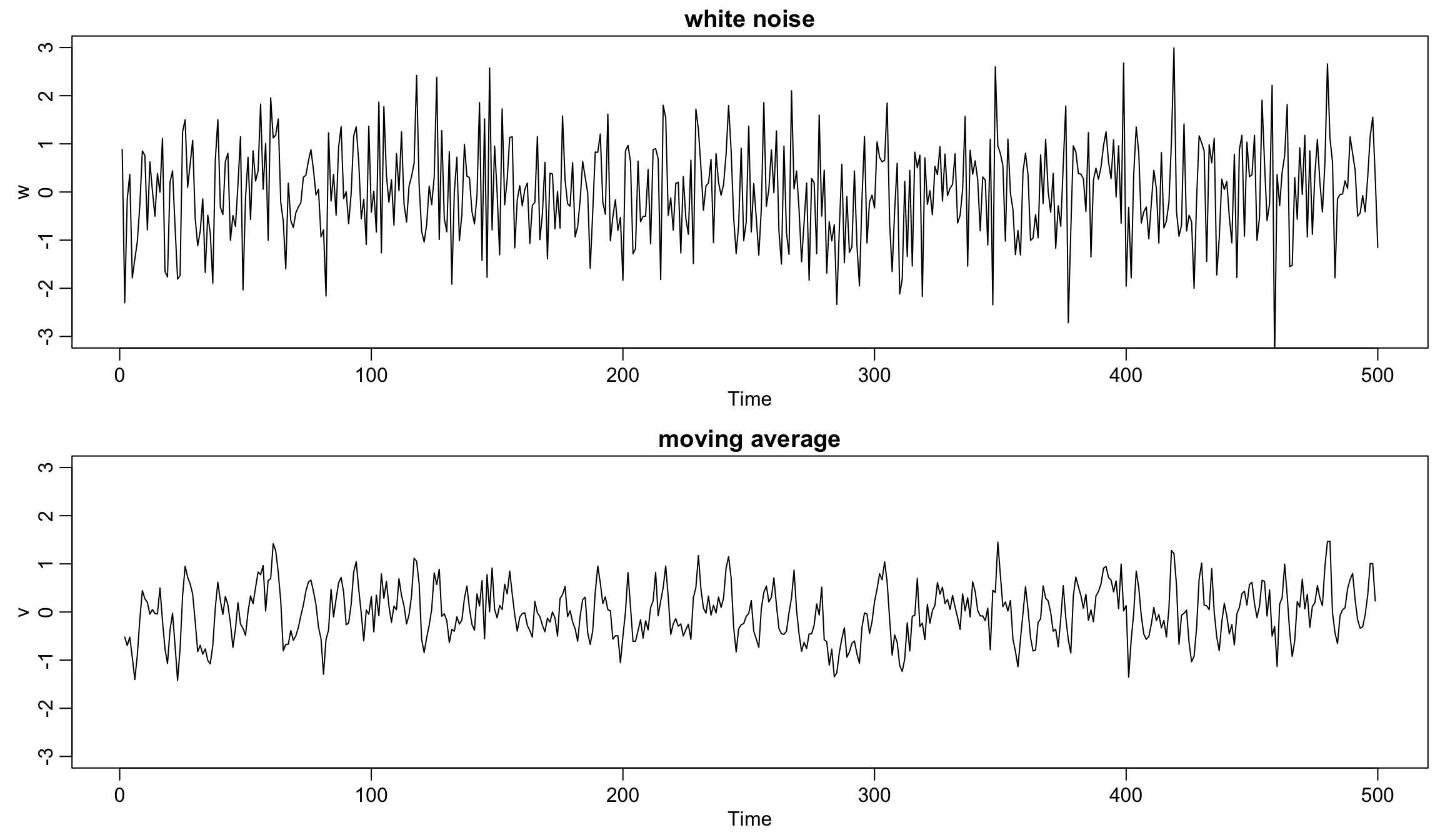
Gaussian white noise series and its 3-point moving average #

w <- rnorm(500, 0, 1)  # 500 N(0,1) variates
plot.ts(w, ylim = c(-3, 3), main = "white noise")
v <- stats::filter(w, sides = 2, filter = rep(1/3, 3))  # moving average
plot.ts(v, ylim = c(-3, 3), main = "moving average")

Filtering (and moving average) #

A series $v_t$ which is a linear combination of values of a more fundamental time series $w_t$ is called a filtered series.

• Example: 3-point moving average (see bottom of previous slide for graph): $$v_t=\frac{1}{3}(w_{t-1}+w_t+w_{t+1}).$$

• In R, moving averages are implemented through the function

  filter(x, filter, method = c("convolution"),sides = 2)
  

  where x is the original series, filter is a vector of weights (in reverse time order), method = c("convolution") is the default (alternative is recursive), and where sides is 1 for past values only, and 2 if weights are centered around lag 0 (requires uneven number of weights).

• Moving average smoothers will be further discussed in Module 8.

Autoregressions #

A series $x_t$ that depends on some of its past values, as well as a noise $w_t$ is called an autoregression, because the formula looks like a regression—not of independent variables, but of its own past values—hence autoregression.

• Example: An autoregression of the white noise: $$x_t=x_{t-1}-0.9x_{t-2}+w_t.$$

• If the autoregression goes back $k$ periods, one needs $k$ initial conditions (filter will use 0’s otherwise).

• In R, autoregressions are implemented through the function

  filter(x, filter, method = c("recursive"),init)
  

  where x is the original series, filter is a vector of weights (reverse time order) and init a vector of initial values (reverse time order).

• Autoregressions will be denoted $AR(p)$ (details in Module 9).

# take this series:
wt <- 1:10
# a simple filter:
filter(wt, rep(1/3, 3), method = c("convolution"), sides = 1)

## Time Series:
## Start = 1 
## End = 10 
## Frequency = 1 
##  [1] NA NA  2  3  4  5  6  7  8  9

# an autoregression
filter(wt, rep(1/3, 3), method = c("recursive"))

## Time Series:
## Start = 1 
## End = 10 
## Frequency = 1 
##  [1]  1.000000  2.333333  4.111111  6.481481  9.308642 12.633745
##  [7] 16.474623 20.805670 25.638012 30.972768

# note how the previous _results_ (rather than wt) are
# being used in the recursion

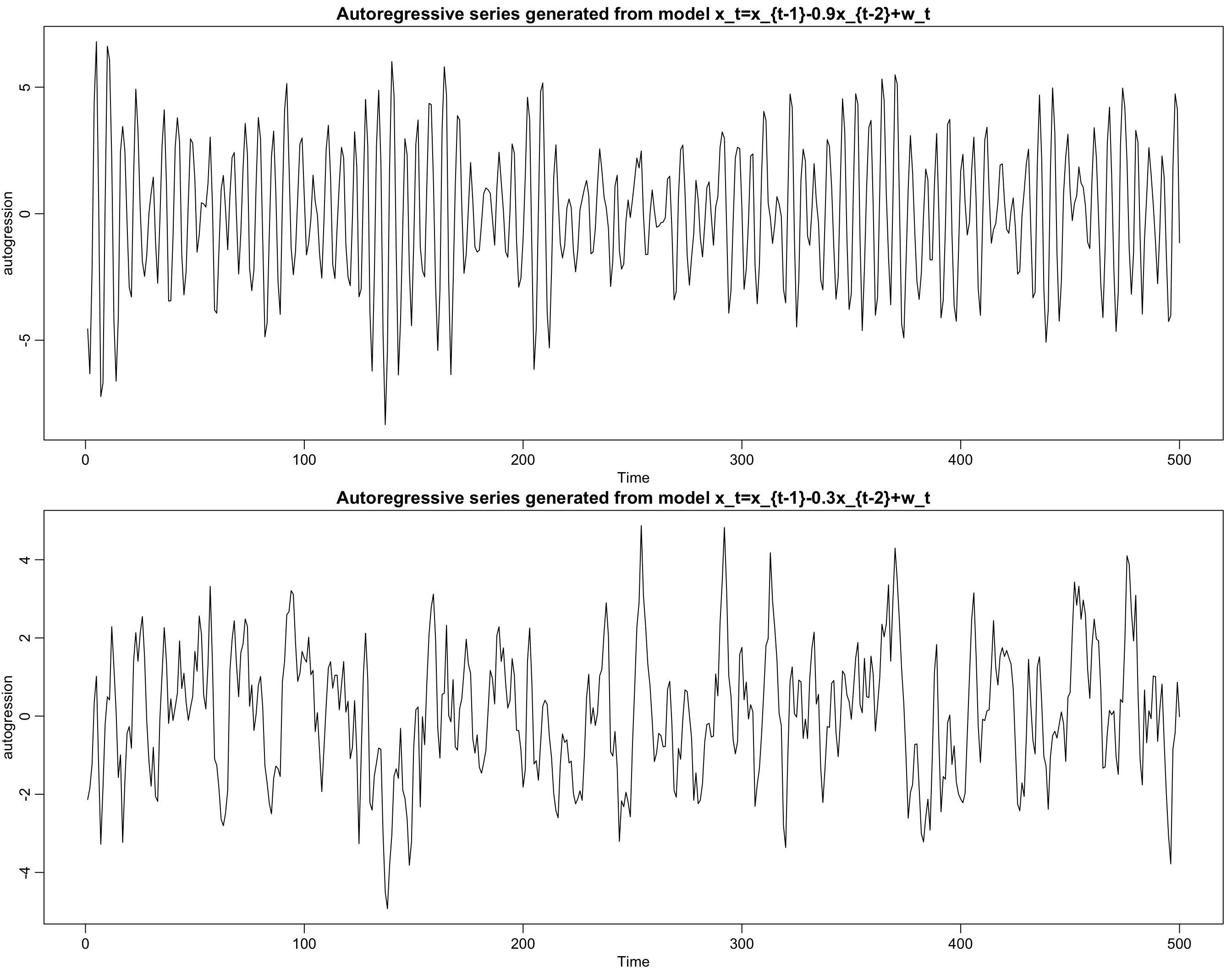
Autoregression examples #

w <- rnorm(550, 0, 1)  # 50 extra to avoid startup problems
x <- stats::filter(w, filter = c(1, -0.9), method = "recursive")[-(1:50)]
# remove first 50
plot.ts(x, ylab = "autogression", main = "Autoregressive series generated from model x_t=x_{t-1}-0.9x_{t-2}+w_t")
y <- stats::filter(w, filter = c(1, -0.3), method = "recursive")[-(1:50)]
# remove first 50
plot.ts(y, ylab = "autogression", main = "Autoregressive series generated from model x_t=x_{t-1}-0.3x_{t-2}+w_t")

Random walk with drift #

• The autoregressions introduced above are all centered around 0 for all $t$ (in the expected sense).
• Assume now that the series increases linearly by $\delta$ (called drift) every time unit.
• The random walk with drift looks back only one time unit: $$x_t=\delta +x_{t-1}+w_t=\delta t+\sum _{j=1}^t{w}_j\text{ for }t=1,2,\dots$$ with initial condition $x_0=0$ and with $w_t$ a white noise.
• If $\delta =0$ this is simply called a random walk.
• The term can be explained by visualising each increment from $t$ to $t+1$ as a purely random step from wherever the process is at $x_t$, ignoring what happened before.

Random walk with drift $\delta =0.2$ and ${\sigma }_w=1$ #

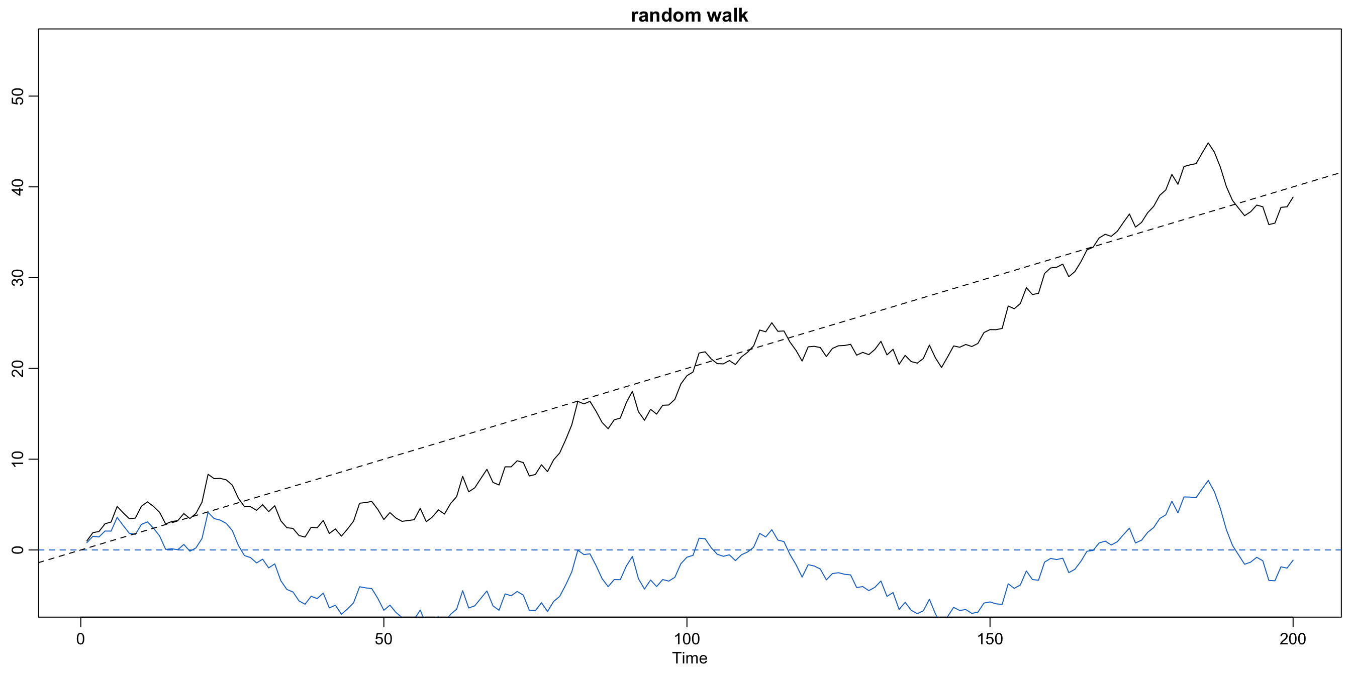
Code used to generate the plot:

set.seed(155)  # so you can reproduce the results
w <- rnorm(200)
x <- cumsum(w)
wd <- w + 0.2
xd <- cumsum(wd)
plot.ts(xd, ylim = c(-5, 55), main = "random walk", ylab = "")
lines(x, col = 4)
abline(h = 0, col = 4, lty = 2)

Describing the behaviour of basic models (TS 1.3) #

Motivation #

• In this section we would like to develop theoretical measures to help describe how times series behave.

• We are particularly interested in describing the relationships between observations at different points in time.

Full specification #

• A full specification of a time series of size $n$ at times $t_1,t_2,\dots ,t_n$ for any $n$ would require the full joint distribution function $$F_{t_1,t_2,\dots ,t_n}(c_1,c_2,\dots ,c_n)=Pr[x_{t_1}\le c_1,x_{t_2}\le c_2,\dots ,x_{t_n}\le c_n].$$ This is a quite unwieldy tool for analysis.
• Examination of the margins $F_t(x)=Pr[x_t\le x]$ and corresponding pdf $f_t(x)$, when they exist, can be informative.
• These are very theoretical. In practice, one often have only one realisation for each $x_t$ so that inferring full distributions (let alone their dependence structure) is simply impractical without tricks, manipulations, and assumptions (some of which we will learn).

What would be the most basic descriptors?

Mean function #

The mean function is defined as $${\mu }_{xt}=E[x_t]={\int }_{-\mathrm{\infty }}^{\mathrm{\infty }}x{f}_t(x)dx.$$

Examples:

• Moving Average Series: we have $${\mu }_{vt}=E[v_t]=\frac{1}{3}(E[w_{t-1}]+E[w_t]+E[w_{t+1}])=0.$$ Smoothing does not change the mean.
• Random walk with drift: we have $${\mu }_{xt}=E[x_t]=\delta t+\sum _{j=1}^{t}E[w_j]=\delta t.$$

Autocovariance function #

The autocovariance function is defined as the second moment product $${\gamma }_x(s,t)=Cov(x_s,x_t)=E[(x_s-{\mu }_{xs})(x_t-{\mu }_{xt})]$$ for all $s$ and $t$. Note:

• We will write ${\gamma }_x(s,t)=\gamma (s,t)$ if no confusion is possible.
• This is a measure of linear dependence.
• Smooth series $\to$ large $\gamma$ even for $t$ and $s$ far apart
• Choppy series $\to$ $\gamma$ is nearly zero for large separations
• [ ${\gamma }_x(s,t)=0$ $⟹$ independence] $⟸$ all variables are normal

For two series $x_t$ and $y_t$ this becomes $${\gamma }_{xy}(s,t)=Cov(x_s,y_t)=E[(x_s-{\mu }_{xs})(y_t-{\mu }_{yt})],$$ called cross-covariance function.

Examples of autocovariance functions #

White noise: The white noise series $w_t$ has $E[w_t]=0$ and $${\gamma }_w(s,t)=Cov(w_s,w_t)=\{\begin{array}{lc}{\sigma }_w^2& s=t\\ 0& s\ne t\end{array}$$

Remember that if $$U=\sum _{j=1}^m{a}_j{X}_j$$ and $$V=\sum _{k=1}^r{b}_k{Y}_k$$ then $$Cov(U,V)=\sum _{j=1}^m\sum _{k=1}^r{a}_j{b}_{k}Cov(X_j,Y_k).$$ This will be useful for computing $\gamma$ of filtered series.

Moving average: A 3-point moving average $v_t$ to the white noise series $w_t$ has $${\gamma }_v(s,t)=Cov(v_s,v_t)=\{\begin{array}{lc}\frac{3}{9}{\sigma }_w^2& s=t\\ \frac{2}{9}{\sigma }_w^2& |s-t|=1\\ \frac{1}{9}{\sigma }_w^2& |s-t|=2\\ 0& |s-t|>2\end{array}$$ This only depends on the time separation lag only, and not on the absolute location along the series.

This is related to the concept of weak stationarity which will introduce later.

Random walk: For the random walk $x_t=\sum _{j=1}^t{w}_j$ we have $$\begin{array}{rcl}{\gamma }_x(s,t)& =& Cov(x_s,x_t)\\ \\ & =& Cov\left({\displaystyle \sum _{j=1}^s{w}_j,\sum _{k=1}^t{w}_k}\right)\\ \\ & =& min\{s,t\}{\sigma }_w^2.\end{array}$$ Contrary to the previous examples, this depends on the absolute location rather than the lag.

Also $Var(x_t)=t{\sigma }_w^2$ increases without bound as $t$ increases.

The autocorrelation function (ACF) #

The autocorrelation function (ACF) is defined as $$-1\le \rho (s,t)=\frac{\gamma (s,t)}{\sqrt{\gamma (s,s)\gamma (t,t)}}\le 1.$$

• The ACF measures the linear predictability of the series at time $t$, say $x_t$, using only the value $x_s$.
• If we could do that perfectly, then $\rho (s,t)\pm 1$ and $$x_t={\beta }_0+{\beta }_1{x}_s$$ with ${\beta }_1$ of same sign as $\rho (s,t)$.

In the case of two series this becomes $$-1\le {\rho }_{xy}(s,t)=\frac{{\gamma }_{xy}(s,t)}{\sqrt{{\gamma }_x(s,s){\gamma }_y(t,t)}}\le 1,$$ called cross-correlation function (CCF).

Stationary time series (TS 1.4) #

Strict stationarity #

A strictly stationary times series is one for which the probabilistic behaviour of every collection of values $\{x_{t_1},x_{t_2},\dots ,x_{t_k}\}$ is identical to that of the time shifted set (for any $h$) $\{x_{t_1+h},x_{t_2+h},\dots ,x_{t_k+h}\}.$ That is, $$Pr[x_{t_1}\le c_1,x_{t_2}\le c_2,\dots ,x_{t_k}\le c_k]$$ $$=Pr[x_{t_1+h}\le c_1,x_{t_2+h}\le c_2,\dots ,x_{t_k+h}\le c_k]$$ for all $k=1,2,\dots$, all the time points $t_1,t_2,\dots ,t_k$, all numbers $c_1,c_2,\dots ,c_k$ and all time shifts $h=0,\pm 1,\pm 2,\dots$. This implies

• identical marginals of dimensions $<k$ for any shift $h$
• constant mean: ${\mu }_{xs}={\mu }_{xt}\equiv \mu$
• for $k=2$, an autocovariance function that depends only on $t-s$: $\gamma (s,t)=\gamma (s+h,t+h)$

We need something less constraining, that still allows us to infer
properties from a single series.

Weak stationarity #

A weakly stationary time series, $x_t$, is a finite variance process such that

1. the mean value function, ${\mu }_{xt}$ is constant and does not depend on time $t$, and
2. the autocovariance function, $\gamma (s,t)$ depends on $s$ and $t$ only through their difference $|s-t|$.

Note:

• We dropped full distributional requirements. This imposes conditions on the first two moments of the series only.
• Since those completely define a normal distribution, a (weak) stationary Gaussian time series is also strictly stationary.
• We will use the term stationary to mean weakly stationary; if a process is stationary in the strict sense, we will use the term strictly stationary.

Stationarity means we can estimate those two quantities by averaging of a single series. This is what we needed.

Properties of stationary series #

• Because of condition 1, $${\mu }_t=\mu .$$

• Because of condition 2, $$\gamma (t+h,t)=Cov(x_{t+h},x_t)=Cov(x_h,x_0)=\gamma (h,0)\equiv \gamma (h)$$ and the autocovariance of a stationary time series is then $$\gamma (h)=Cov(x_{t+h},x_t)=E[(x_{t+h}-\mu )(x_t-\mu )].$$

• $\gamma (h)$ is non-negative definite, which means that the variance of linear combinations of variates $x_t$ will never be negative, that is, $$0\le Var(a_1{x}_1+\cdots +a_n{x}_n)=\sum _{j=1}^n\sum _{k=1}^n{a}_j{a}_k\gamma (j-k).$$

• Furthermore, $$|\gamma (h)|\le \gamma (0)\text{ (the variance of the time series)}$$ and $$\gamma (h)=\gamma (-h).$$
• The autocorrelation function (ACF) of a stationary time series becomes $$-1\le \rho (h)=\frac{\gamma (t+h,t)}{\sqrt{\gamma (t+h,t+h)\gamma (t,t)}}=\frac{\gamma (h)}{\gamma (0)}\le 1.$$

Examples of (non)-stationarity #

White noise: We have $${\mu }_{wt}=0$$ and $${\gamma }_w(h)=Cov(w_{t+h},w_t)=\{\begin{array}{lc}{\sigma }_w^2& h=0,\\ 0& h\ne 0,\end{array},$$ which are both independent of time. Hence, the white noise satisfies both conditions and is (weakly) stationary. Furthermore, $${\rho }_w(h)=\{\begin{array}{lc}1& h=0,\\ 0& h\ne 0.\end{array}$$ If in addition $w_t\sim \text{iid N}(0,{\sigma }_w^2)$, then it is also strictly stationary.

Moving average: For the 3-point MA we have $${\mu }_{vt}=0\text{ and }{\gamma }_v(h)=\{\begin{array}{lc}\frac{3}{9}{\sigma }_w^2& h=0,\\ \frac{2}{9}{\sigma }_w^2& h\pm 1,\\ \frac{1}{9}{\sigma }_w^2& h\pm 2,\\ 0& |h|>2,\end{array}$$ which are both independent of time. Hence, the 3-point MA satisfies both conditions and is stationary. Furthermore, $${\rho }_v(h)=\{\begin{array}{lc}1& h=0,\\ \frac{2}{3}& h\pm 1,\\ \frac{1}{3}& h\pm 2,\\ 0& |h|>2,\end{array}$$ which is symmetric around lag 0.

Random walk: For the random walk model $x_t=\sum _{j=1}^t{w}_j$ we have $${\mu }_{xt}=\delta t,$$ which is a function of time $t$, and $$\gamma (s,t)=min\{s,t\}{\sigma }_w^2,$$ which depends on $s$ and $t$ (not just their difference), so the random walk is not stationary.

Furthermore, remember $$Var(x_t)={\gamma }_x(t,t)=t{\sigma }_w^2$$ which increases without bound as $t\to \mathrm{\infty }$.

Trend stationarity #

• If only the second condition (on the ACF) is satisfied, but not the first condition (on the mean value function), we have trend stationarity
• This means that the model has a stationary behaviour around its trend.
• Example: if $$x_t=\alpha +\beta t+y_t\text{where }{y}_t\text{ is stationary,}$$ then the mean function is $${\mu }_{x,t}=E[x_t]=\alpha +\beta t+{\mu }_y,$$ which is *not* independent of time. The autocovariance function, $$\begin{array}{rcl}{\gamma }_x(h)=Cov(x_{t+h},x_t)& =& E[(x_{t+h}-{\mu }_{x,t+h})(x_t-{\mu }_{x,t})]\\ \\ & =& E[(y_{t+h}-{\mu }_y)(y_t-{\mu }_y)]={\gamma }_y(h),\end{array}$$ however, is independent of time.

Joint stationarity #

Two time series, say, $x_t$ and $y_t$, are said to be jointly stationary if they are each stationary, and the cross-covariance function $${\gamma }_{xy}(h)=Cov(x_{t+h},y_t)=E[(x_{t+h}-{\mu }_x)(y_t-{\mu }_y)]$$ is a function only of lag $h$. The corresponding cross-correlation function (CCF) is $$1\le {\rho }_{xy}(h)=\frac{{\gamma }_{xy}(h)}{\sqrt{{\gamma }_x(0){\gamma }_y(0)}}\le 1.$$

Note that because $Cov(x_2,y_1)$ and $Cov(x_1,y_2)$ (for example) need not be the same, it follows that typically $${\rho }_{xy}(h)\ne {\rho }_{xy}(-h),$$ that is, the CCF is not generally symmetric about zero. However, we have $${\rho }_{xy}(h)={\rho }_{yx}(-h).$$

Example of joint stationarity #

Consider $$x_t=w_t+w_{t-1}\text{and}{y}_t=w_t-w_{t-1},$$ where $w_t$ are independent with mean 0 and variance ${\sigma }_w^2$. We have then $$\begin{array}{rcl}{\gamma }_x(0)& =& {\gamma }_y(0)=2{\sigma }_w^2\\ {\gamma }_x(-1)& =& {\gamma }_x(1)={\sigma }_w^2\\ {\gamma }_y(-1)& =& {\gamma }_y(1)=-{\sigma }_w^2\end{array}$$ and $${\gamma }_{xy}(-1)=-{\sigma }_w^2,{\gamma }_{xy}(0)=0,\text{ and }{\gamma }_{xy}(1)={\sigma }_w^2,$$ so that $${\rho }_{xy}(h)=\{\begin{array}{cl}0& h=0,\\ 1/2& h=1,\\ -1/2& h=-1,\\ 0& |h|\ge 2,\end{array}$$ which depends only on the lag $h$, so both series are jointly stationary.

Prediction using cross-correlation #

Prediction using cross-correlation: A lagging relation between two series $x_t$ and $y_t$ may be exploited for predictions. For instance, if $$y_t=A{x}_{t-\ell }+w_t,$$ $x_t$ is said to lead $y_t$ for $\ell >0$, and is said to lag $y_t$ for $\ell <0$.

If the relation above holds true, then the lag $\ell$ can be inferred from the shape of the autocovariance of the input series $x_t$:

• If $w_t$ is uncorrelated with $x_t$ then $$\begin{array}{rcl}{\gamma }_{yx}(h)& =& Cov(y_{t+h},x_t)=Cov(A{x}_{t+h-\ell }+w_{t+h},x_t)\\ & =& Cov(A{x}_{t+h-\ell },x_t)=A{\gamma }_x(h-\ell )\end{array}$$
• We know $${\gamma }_x(h-\ell )\le {\gamma }_x(0),$$ and the peak of ${\gamma }_{yx}(h)$ should be at $h=\ell$. Also:
  $h$ will be positive if $x_t$ leads $y_t$, negative if $x_t$ lags $y_t$.

• Here $\ell =5$ and $x_t$ leads $y_t$:

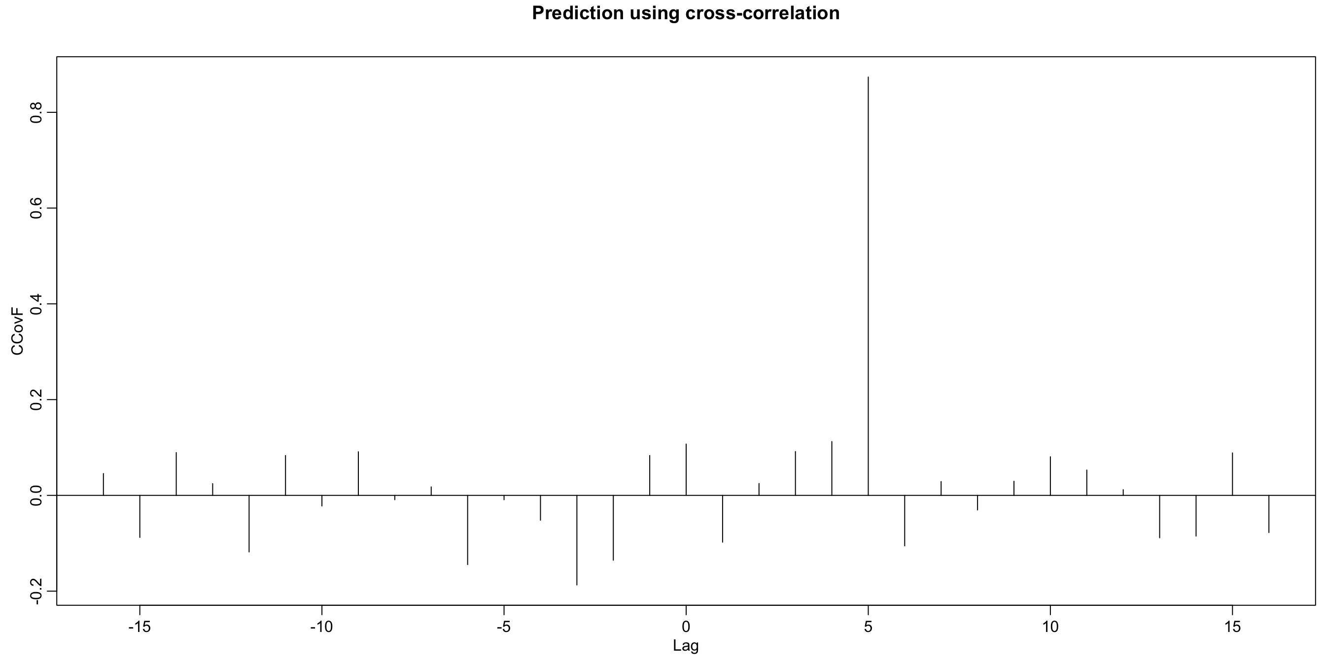
Note this example was simulated and uses the R functions lag and ccf:

x <- rnorm(100)
y <- stats::lag(x, -5) + rnorm(100)
ccf(y, x, ylab = "CCovF", type = "covariance")

Linear process #

A linear process, $x_t$ , is defined to be a linear combination of white noise variates $w_t$, and is given by $$x_t=\mu +\sum _{j=-\mathrm{\infty }}^{\mathrm{\infty }}{\Psi }_j{w}_{t-j},\sum _{j=-\mathrm{\infty }}^{\mathrm{\infty }}|{\Psi }_j|<\mathrm{\infty }$$ This is an important class of models because it encompasses moving averages, autoregressions, and also the combination of both, called autoregressive moving average (ARMA) processes which we will introduce later.

Example:

• Moving average The 3-point moving average has $${\Psi }_0={\Psi }_{-1}={\Psi }_1=1/3$$ and is hence a linear process.

Properties of linear processes #

• The autocovariance function of a linear process is given by $${\gamma }_x(h)={\sigma }_w^2\sum _{j=-\mathrm{\infty }}^{\mathrm{\infty }}{\Psi }_{j+h}{\Psi }_j\text{for }h\ge 0.$$
• It has finite variance if $\sum _{j=-\mathrm{\infty }}^{\mathrm{\infty }}{\Psi }_j^2<\mathrm{\infty }$.
• In its most general form $x_t$ depends on the future ($j<0$ components), the present ($j=0$) and the past ($j>0$).

For forecasting, a model dependent on the future is useless. We will focus on processes that do not depend on the future. Such processes are called causal, that is, $$x_t\text{ is causal}⟺{\Psi }_j=0\text{ for }j<0,$$ which we will assume unless stated otherwise.

Estimation of correlation (TS 1.5) #

Background #

• One can very rarely hypothetise (specify) time series. In practice, most analyses are performed using sample data.
• Furthermore, one often has only one realisation of the time series.
• This means that we don’t have $n$ realisations of the time series to estimate its covariance and correlation functions.
• This is why the assumption of stationarity is essential: in this case, the assumed `homogeneity’ of the data means we can estimate those functions on one realisation only.
• This also means that one needs to manipulate / de-trend series such that they are arguably stationary before we can fit parameters to them and use them for projections.

Sample mean #

If a time series is stationary the mean function ${\mu }_t=\mu$ is constant so that we can estimate it by the sample mean, $$\bar{x}=\frac{1}{n}\sum _{t=1}^n{x}_t.$$ This estimator is unbiased, $$E[\bar{x}]=\mu ,$$ and has standard error the square root of $$Var(\bar{x})=\frac{1}{n^2}Cov(\sum _{t=1}^n{x}_t,\sum _{s=1}^n{x}_s)=\frac{1}{n}\sum _{h=-n}^n(1-\frac{|h|}{n}){\gamma }_x(h).$$

Sample autocovariance function #

The sample autocovariance function is defined as $$\hat{\gamma }(h)=\frac{1}{n}\sum _{t=1}^{n-h}(x_{t+h}-\bar{x})(x_t-\bar{x})\text{with }\hat{\gamma }(-h)=\hat{\gamma }(h)\text{ for }h=0,1,\dots ,n-1.$$ Note:

• The estimator is biased.
• The sum runs over a restricted range ($n-h$) because $x_{t+h}$ is not available for $t+h>n$.
• One could wonder why the factor of the sum is not $1/(n-h)$ (the number of elements in the sum), but factor $1/n$ is not a mistake. It ensures that the estimate of the variances of linear combinations, $$\widehat{Var}(a_1{x}_1+\cdots +a_n{x}_n)=\sum _{j=1}^n\sum _{k=1}^n{a}_j{a}_k\hat{\gamma }(j-k),$$ is non-negative.

Sample autocorrelation function #

The sample autocorrelation function (SACF) is $$\hat{\rho }(h)=\frac{\hat{\gamma }(h)}{\hat{\gamma }(0)}.$$

Under some conditions (see book for details), if $x_t$ is a white noise, then for large $n$, the SACF $\hat{\rho }(h)$ is approximately normally distributed with zero mean and standard deviation given by $${\sigma }_{\hat{\rho }(h)}=\frac{1}{\sqrt{n}}.$$

Testing for significance of autocorrelation #

The asymptotic result for the variance of the SACF means we can test whether lagged observations are uncorrelated (which is a requirement for white noise):

• test for significance of the $\hat{\rho }$’s at different lags: check how many $\hat{\rho }$’s lie outside the interval $\pm 2/\sqrt{n}$ (a 95% confidence interval)
• One should expect approximately 1 out of 20 to lie outside the interval if the sequence is a white noise. Many more than that would invalidate the whiteness assumption.
• This allows for a recursive approach for manipulating / de-trending series until they are white noise, called whitening.
• The R function acf automatically displays those bounds with dashed blue lines.

SOI autocorrelation #

acf(soi, main = "Sample autocorrelation function (SACF) of SOI")

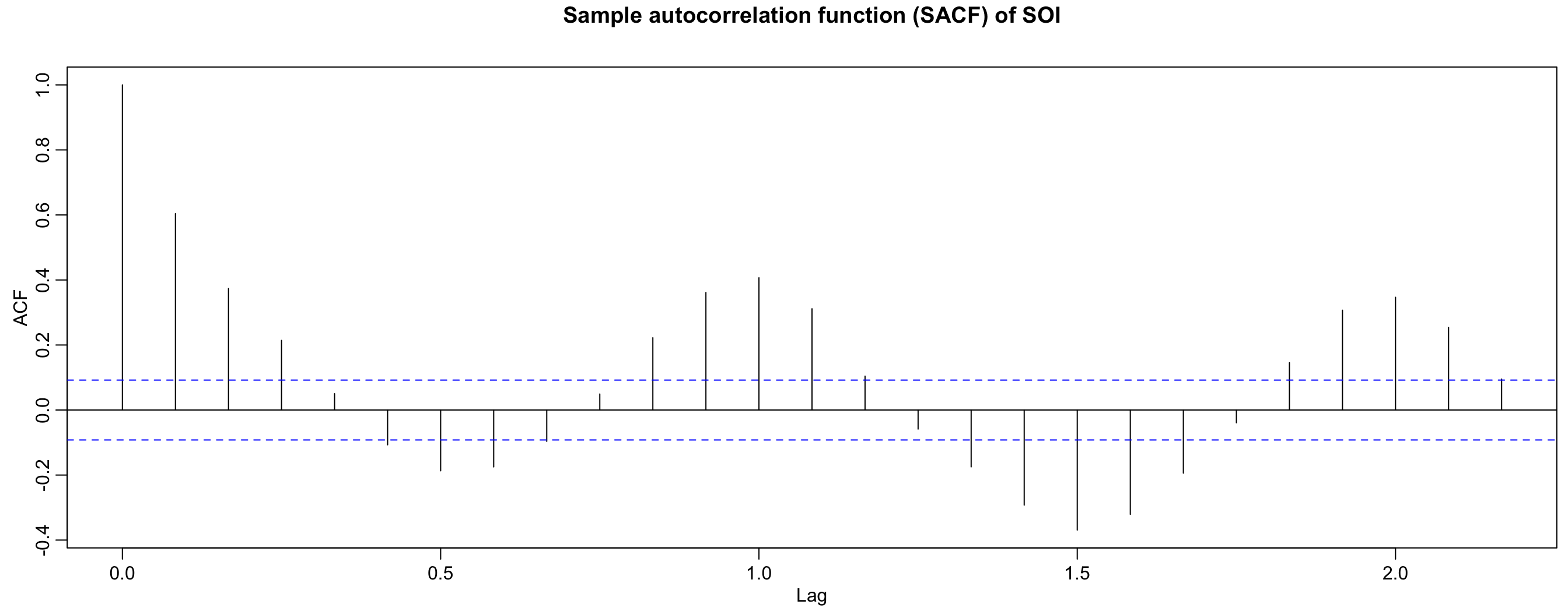
r <- round(acf(soi, 6, plot = FALSE)$acf[-1], 3)  # first 6 sample acf values

## [1]  0.604  0.374  0.214  0.050 -0.107 -0.187

The SOI series is clearly not a white noise.

plot(stats::lag(soi, -1), soi, main = "SOI pairs of values 1 month apart")
legend("topleft", legend = r[1])
plot(stats::lag(soi, -6), soi, main = "SOI pairs of values 6 months apart")
legend("topleft", legend = r[6])

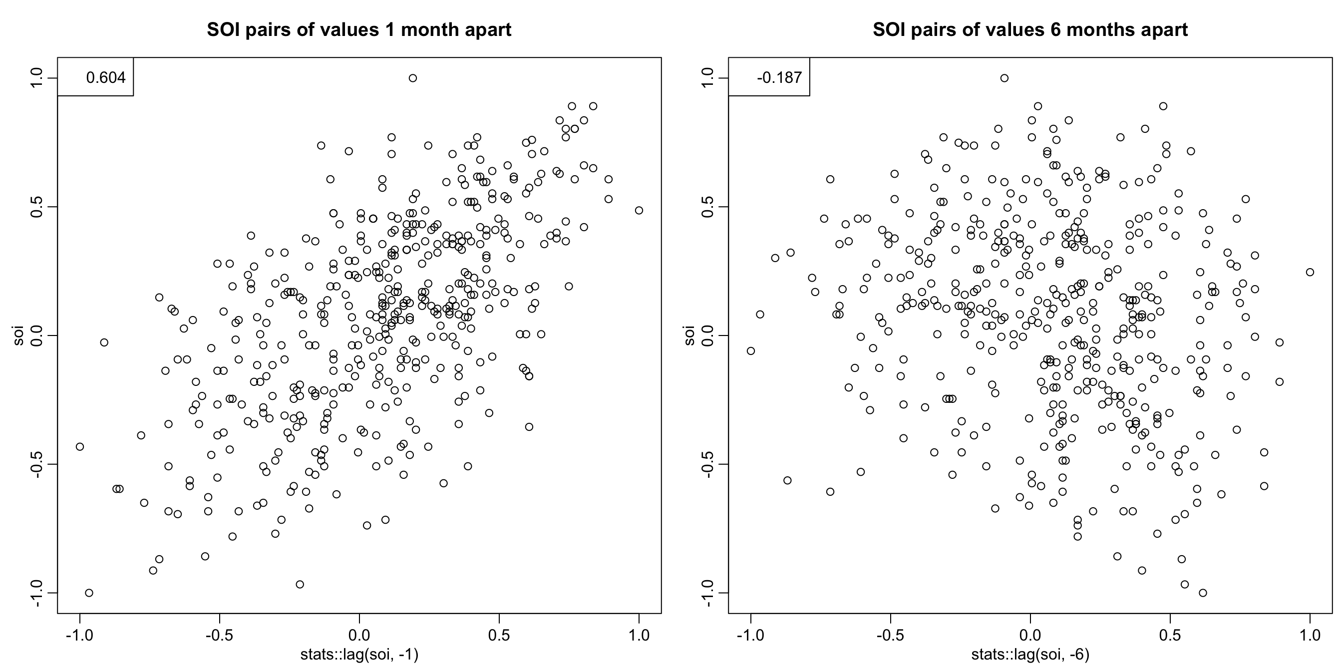
Scatterplots allow to have a visual representation of the dependence
(which may not necessarily be linear).

Sample cross-covariances and cross-correlations #

The sample cross-covariance function is $${\hat{\gamma }}_{xy}(h)=\frac{1}{n}\sum _{t=1}^{n-h}(x_{t+h}-\bar{x})(y_t-\bar{y}),$$ where ${\hat{\gamma }}_{xy}(-h)={\hat{\gamma }}_{yx}(h)$ determines the function for negative lags.

The sample cross-correlation function is $$-1\le {\hat{\rho }}_{xy}(h)=\frac{{\hat{\gamma }}_{xy}(h)}{\sqrt{{\hat{\gamma }}_x(0){\hat{\gamma }}_y(0)}}\le 1.$$ Note:

• Graphical examinations of ${\hat{\rho }}_{xy}(h)$ provide information about the leading or lagging relations in the data.

Testing for independent cross-whiteness #

If $x_t$ and $y_t$ are independent linear processes then the large sample distribution of ${\hat{\rho }}_{xy}(h)$ has mean 0 and $${\sigma }_{{\hat{\rho }}_{xy}}=\frac{1}{\sqrt{n}}$$ if at least one of the processes is independent white noise.

This is very useful, and adds to the toolbox:

• This provides feedback about the quality of our explanation of the relationship between both time series: if we have explained the trends and relationships between both processes, then their residuals should be independent white noise.
• After each improvement of our model, significance of the ${\hat{\rho }}_{xy}$’s of the residuals can be tested: if we have independent cross-whiteness then we have a good model. If the ${\hat{\rho }}_{xy}$’s are still significant (outside
  the boundaries) then we still have things to explain (to add).

SOI and recruitment correlation analysis #

acf(soi, 48, main = "Southern Oscillation Index")
acf(rec, 48, main = "Recruitment")
ccf(soi, rec, 48, main = "SOI vs Recruitment", ylab = "CCF")

The SCCF (bottom) has a different cycle, and peak at $h=-6$
suggests SOI leads Recruitment by 6 months (negatively).

Idea of prewhitening #

• to use the test of cross-whiteness one needs to “prewhiten” at least one of the series
• for the SOI vs recruitment example, there is strong seasonality which, upon removal, may whiten the series
• we look at an example here that looks like the SOI vs recruitment example, and show how this seasonality could be removed with the help of $\sin$ and $\cos$ functions

Example:

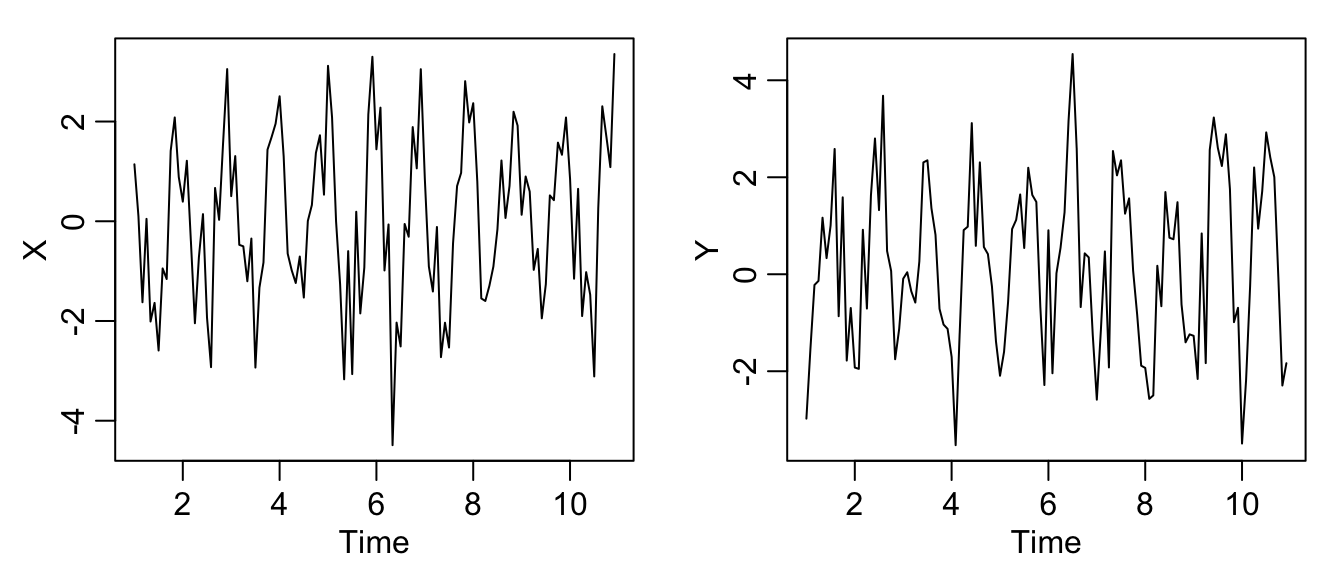
• Let us generate two series $x_t$ and $y_t$, for $t=1,\dots ,120$, independently as $$x_t=2\cos \left(2\pi t\frac{1}{12}\right)+w_{t1}\text{and}{y}_t=2\cos (2\pi [t+5])\frac{1}{12})+w_{t2},$$ where $\{w_{t1},w_{t2};t=1,\dots ,120\}$ are all independent standard
  normals.

• this generates the data and plots it:

set.seed(1492)
num <- 120
t <- 1:num
X <- ts(2 * cos(2 * pi * t/12) + rnorm(num), freq = 12)
Y <- ts(2 * cos(2 * pi * (t + 5)/12) + rnorm(num), freq = 12)
par(mfrow = c(1, 2), mgp = c(1.6, 0.6, 0), mar = c(3, 3, 1, 1))
plot(X)
plot(Y)

• looking at the ACFs one can see seasonality

par(mfrow = c(3, 2), mgp = c(1.6, 0.6, 0), mar = c(3, 3, 1, 1))
acf(X, 48, ylab = "ACF(X)")
acf(Y, 48, ylab = "ACF(Y)")
ccf(X, Y, 24, ylab = "CCF(X,Y)")

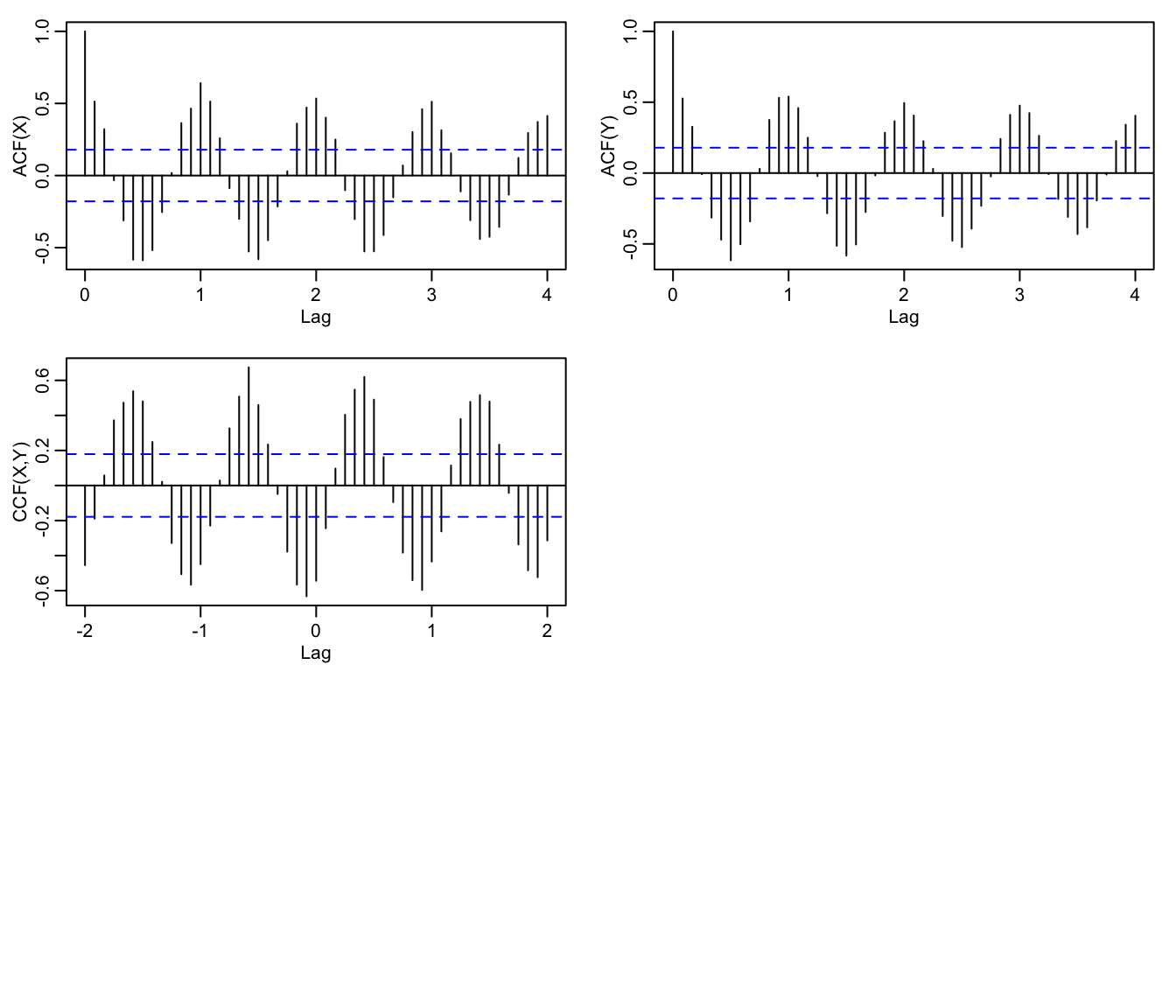
• furthermore the CCF suggests cross-correlation
  even though the series are independent

• what we do now is to “prewhiten” $y_t$ by removing the signal from the data by running a regression of $y_t$ on $\cos (2\pi t)$ and $\sin (2\pi t)$ and then putting $$\tilde{y}=y_t-{\hat{y}}_t,$$ where ${\hat{y}}_t$ are the predicted values from the regression.
• in the R code below, Yw is $\tilde{y}$

par(mgp = c(1.6, 0.6, 0), mar = c(3, 3, 1, 1))
Yw <- resid(lm(Y ~ cos(2 * pi * t/12) + sin(2 * pi * t/12), na.action = NULL))
ccf(X, Yw, 24, ylab = "CCF(X,Yw)", ylim = c(-0.3, 0.3))

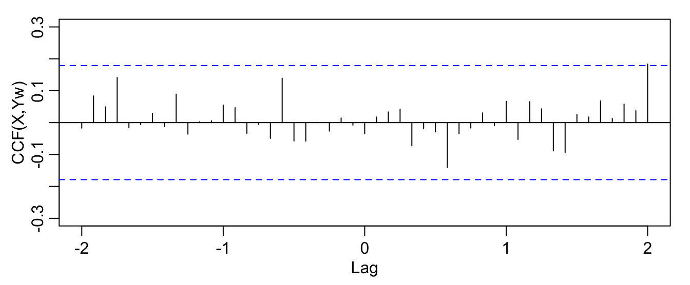
• the updated CCF now suggests cross-independence, as it should

References #