Estimation #
Summary: analysing the ACF and PACF #
Behaviour of the ACF and PACF for ARMA Models #
\(AR(p)\) |
\(MA(q)\) |
\(ARMA(p,q)\) |
|
|---|---|---|---|
| ACF | Tails off | Cuts off after lag \(q\) |
Tails off |
| PACF | Cuts off after lag \(p\) |
Tails off | Tails off |
- The PACF for MA models behaves much like the ACF for AR models.
- The PACF for AR models behaves much like the ACF for MA models.
- Because an invertible ARMA model has an infinite AR representation, its PACF will not cut off.
- Remember that the data might have to be detrended and/or transformed first (e.g., to stabilise the variance, apply a log transform), before such analysis is performed.
Example: Recruitment Series #
acf2(rec, 48) # will produce values and a graph
##      [,1]  [,2]  [,3]  [,4] [,5]  [,6]  [,7] [,8] [,9] [,10] [,11]
## ACF  0.92  0.78  0.63  0.48 0.36  0.26  0.18 0.13 0.09  0.07  0.06
## PACF 0.92 -0.44 -0.05 -0.02 0.07 -0.03 -0.03 0.04 0.05 -0.02 -0.05
##      [,12] [,13] [,14] [,15] [,16] [,17] [,18] [,19] [,20] [,21]
## ACF   0.02 -0.04 -0.12 -0.19 -0.24 -0.27 -0.27 -0.24 -0.19 -0.11
## PACF -0.14 -0.15 -0.05  0.05  0.01  0.01  0.02  0.09  0.11  0.03
##      [,22] [,23] [,24] [,25] [,26] [,27] [,28] [,29] [,30] [,31]
## ACF  -0.03  0.03  0.06  0.06  0.02 -0.02 -0.06 -0.09 -0.12 -0.13
## PACF -0.03 -0.01 -0.07 -0.12 -0.03  0.05 -0.08 -0.04 -0.03  0.06
##      [,32] [,33] [,34] [,35] [,36] [,37] [,38] [,39] [,40] [,41]
## ACF  -0.11 -0.05  0.02  0.08  0.12  0.10  0.06  0.01 -0.02 -0.03
## PACF  0.05  0.15  0.09 -0.04 -0.10 -0.09 -0.02  0.05  0.08 -0.02
##      [,42] [,43] [,44] [,45] [,46] [,47] [,48]
## ACF  -0.03 -0.02  0.01  0.06  0.12  0.17  0.20
## PACF -0.01 -0.02  0.05  0.01  0.05  0.08 -0.04
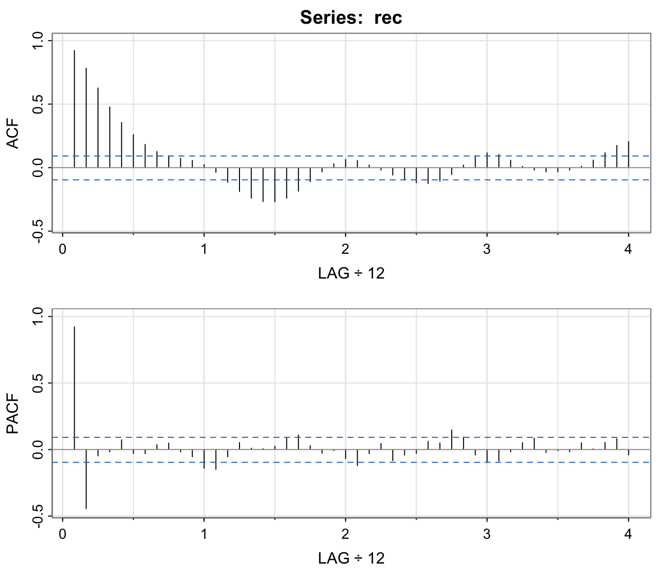
- The behaviour of the PACF is consistent with the behaviour of an AR(2): the ACF tails off, the PACF cuts after lag 2.
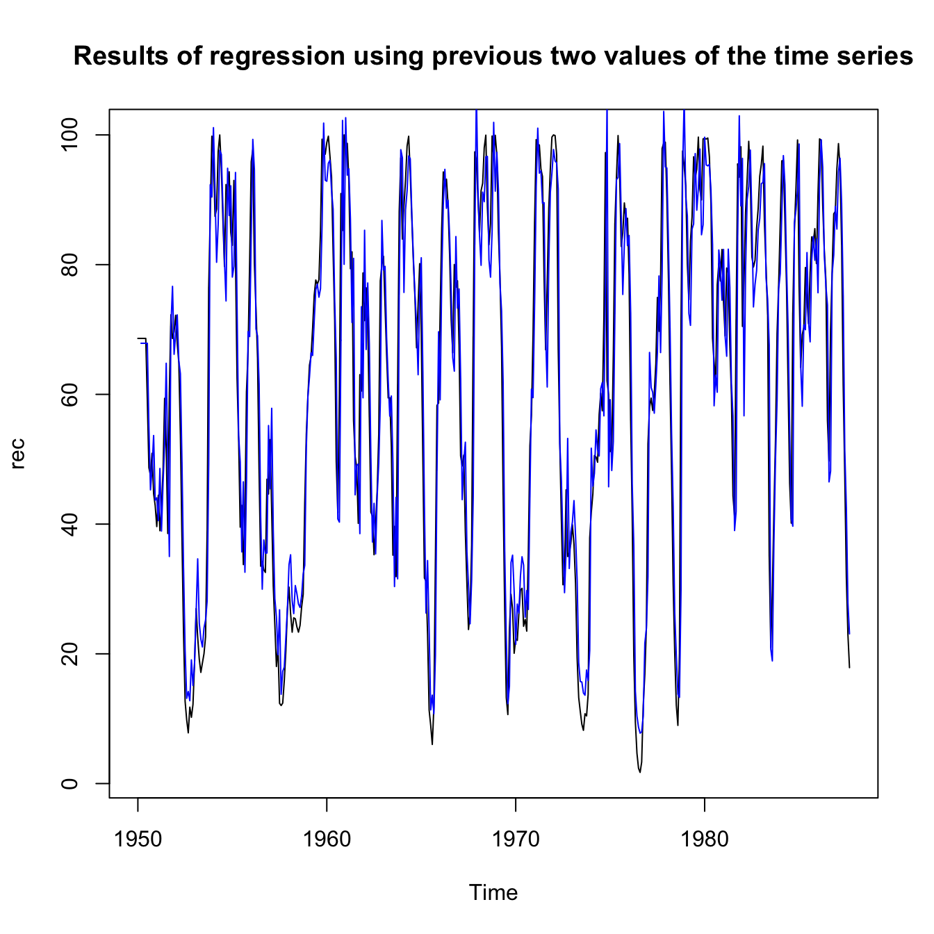
- The following slide shows the fit of a regression using the data triplets
\(\{(x:z_1,z_2): (x_3;x_2,x_1),(x_4;x_3,x_2),\ldots,(x_{447};x_{446},x_{445})\}\)to fit a model of the form$$x_t=\phi_0+\phi_1 x_{t-1}+\phi_2 x_{t-2}+w_t \text{ for }t=3,4,\ldots,447$$ - Let us fit this to an AR process using
ar.ols, which, according to R, willFit an autoregressive time series model to the data by ordinary least squares, by default selecting the complexity by AIC. - Note that the “optimal” order will be chose up to a maximum defined by
orderin the function.
regr <- ar.ols(rec, order = 10, demean = FALSE, intercept = TRUE)
regr
##
## Call:
## ar.ols(x = rec, order.max = 10, demean = FALSE, intercept = TRUE)
##
## Coefficients:
##       1        2
##  1.3541  -0.4632
##
## Intercept: 6.737 (1.111)
##
## Order selected 2  sigma^2 estimated as  89.72
regr$asy.se.coef  # standard errors of the estimates
## $x.mean
## [1] 1.110599
##
## $ar
## [1] 0.04178901 0.04187942
ts.plot(rec, main = "Results of regression using previous two values of the time series")
lines(time(rec)[-c(1, 2)], regr$x.intercept + regr$ar[1] * rec[-c(1,
  length(rec))] + regr$ar[2] * rec[-c(length(rec) - 1, length(rec))],
  col = "blue", lwd = 1)
ACF and PACF in presence of seasonality #
\(AR(P)_s\) |
\(MA(Q)_s\) |
\(ARMA(P,Q)_s\) |
|
|---|---|---|---|
| ACF* | Tails off at lags \(ks\) |
Cuts off after | Tails off at |
\(k=1,2,\ldots,\) |
lag \(Qs\) |
lags \(ks\) |
|
| PACF* | Cuts off after | Tails off at lags \(ks\) |
Tails off at |
lag \(Ps\) |
\(k=1,2,\ldots,\) |
lags \(ks\) |
*The values at nonseasonal lags \(h\neq ks\), for \(k=1,2,\dots,\) are zero.
- This can be seen as a generalisation of the previous table
(which is the special case
\(s=1\)) - Fitting seasonal autoregressive and moving average components first generally leads to more satisfactory results
The Box-Jenkins methodology #
Overview - The Box-Jenkins methodology #
- Determine the integration order
\(d\)of the\(ARIMA(p,d,q)\)and work on the corresponding\(ARMA(p,q)\)by differencing. - Then choose candidates for
\(p\)and\(q\)from examining ACF and PACF - For fixed
\(p\)and\(q\)(candidates), estimate parameters via:
- Method of moments
- Maximum likelihood (Note MLE is more involved than the Method of moments, but way more efficient when
\(q>0\).) - Least squares and variations
- Perform diagnostics, to choose the best
\(p\)and\(q\). This may suggest new candidates for\(p\)and\(q\), in which case we perform a new iteration from step 2. - Use the chosen model for forecasting.
This general approach to fitting is called
the Box-Jenkins methodology.
\(ARIMA(p,d,q) \rightarrow ARMA(p,q)\): choosing \(d\)
#
Choosing \(d\) involves:
- A time series
\(x_t\)may be modelled by a stationary ARMA model if the sample ACF decays rapidly. If the decay is slow (and the ACF is positive) then this suggests further differencing. - Let
\(\sigma_d^2\)be the sample variance of the\(\nabla^d x_t\). This quantity should first decrease with\(d\)until stationarity is achieved, and then starts to increase. Hence\(d\)could be set to the value which minimises\(\sigma_d^2\),\(d\ge 0\).
Several candidates could be selected, a final choice of which could be made after full estimation of all candidates and based on diagnostics.
One should be careful to not over-difference, as this introduces artificial dependence in the data.
Example: Recruitment series #
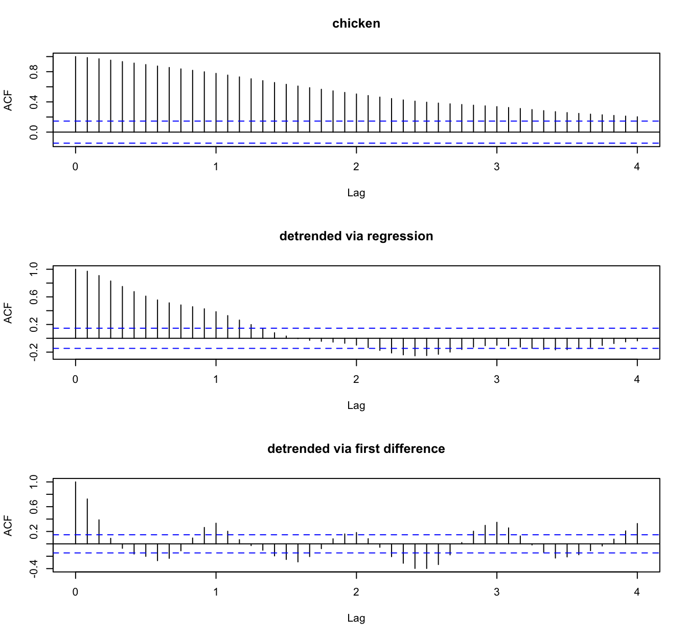
Example: Chicken prices #
Choosing \(p\) and \(q\) for the \(ARMA(p,q)\)
#
- We work on the differenced series, which is then assumed to be
\(ARMA(p,q)\). - We assume the mean of the differenced series is 0. If it isn’t the case in the data, subtract its sample mean, and work on the residuals.
- Examine ACF and PACF to choose candidates for
\(p\)and\(q\):\(p\)can be inferred from the number of spikes in the PACF until a geometrical decay to zero is observed.\(q\)can be inferred from the number of spikes in the ACF until a geometrical decay to zero is observed.
- Alternatively or additionally, work iteratively from the simplest models and increase orders
\(p\)and\(q\):- Higher orders will always reduce the sum of squares (more parameters). At the extreme a model with
\(n\)parameters will replicate the data. - The appropriate order could be chosen using information criteria (e.g., BIC or AIC).
- Higher orders will always reduce the sum of squares (more parameters). At the extreme a model with
Example: Recruitment series #
Estimation of the parameters #
- We now need estimates for
\(\phi_1,\ldots,\phi_p\)and\(\theta_1, \ldots,\theta_q\)for given\(p\)and\(q\) - Use R to fit the model with the function
fit <- arima(x,order=c(p,0,q))wherexis the differenced time series, and wherepandqneed to replaced by their chosen numerical values. The default estimation procedure (unless there are missing values) is to use conditional sum-of-squares to find starting values, then maximum likelihood. - This will output parameter estimates, their standard errors, as well as
\(\sigma^2\)and the AIC. - (One could alternatively use a method of moments approach (see later), but this is much less efficient than MLE if
\(q>0\).)
Example: Recruitment series #
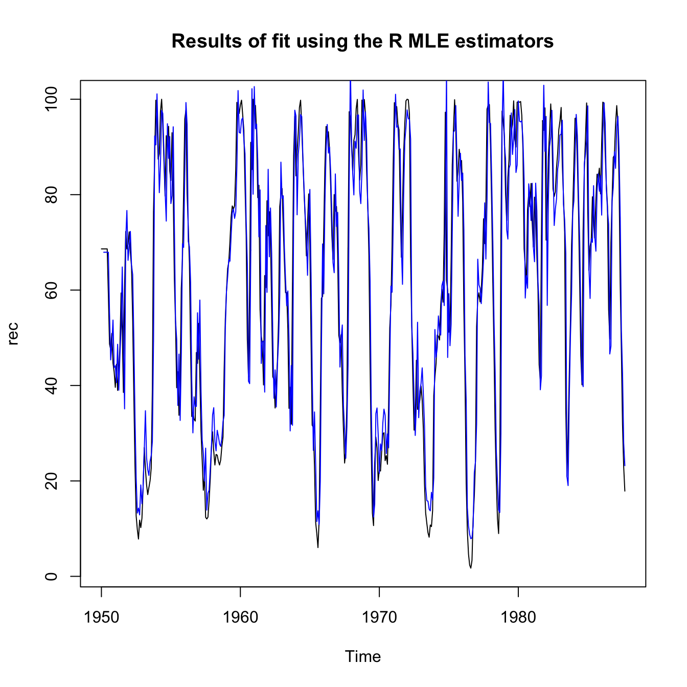
MLE estimators are implemented in R as follows:
rec.mle <- ar.mle(rec, order = 2)
rec.mle$x.mean
## [1] 62.26153
rec.mle$ar
## [1]  1.3512809 -0.4612736
sqrt(diag(rec.mle$asy.var.coef))
## [1] 0.04099159 0.04099159
rec.mle$var.pred
## [1] 89.33597
and then the fit is displayed as follows:
ts.plot(rec, main = "Results of fit using the R MLE estimators")
lines(rec[1:length(rec)] - rec.mle$resid, col = "blue", lwd = 1)
The best R estimators are implemented in R as follows:
rec.arima0 <- arima(rec, order = c(2, 0, 0))  # to use with tsdiag
rec.arima <- sarima(rec, 2, 0, 0)
rec.arima0$coef[3]  # 61.86
## intercept
##  61.85847
rec.arima0$coef[1:2]  # 1.35, -.46
##        ar1        ar2
##  1.3512196 -0.4612128
sqrt(diag(rec.arima0$var.coef))  # .04, .04
##        ar1        ar2  intercept
## 0.04158461 0.04166812 4.00393378
rec.arima0$sigma2  # 89.33
## [1] 89.33436
and then the fit is displayed as follows:
ts.plot(rec, main = "Results of fit using the R ARIMA estimators")
lines(rec[1:length(rec)] - rec.arima$fit$residuals, col = "blue",
  lwd = 1)

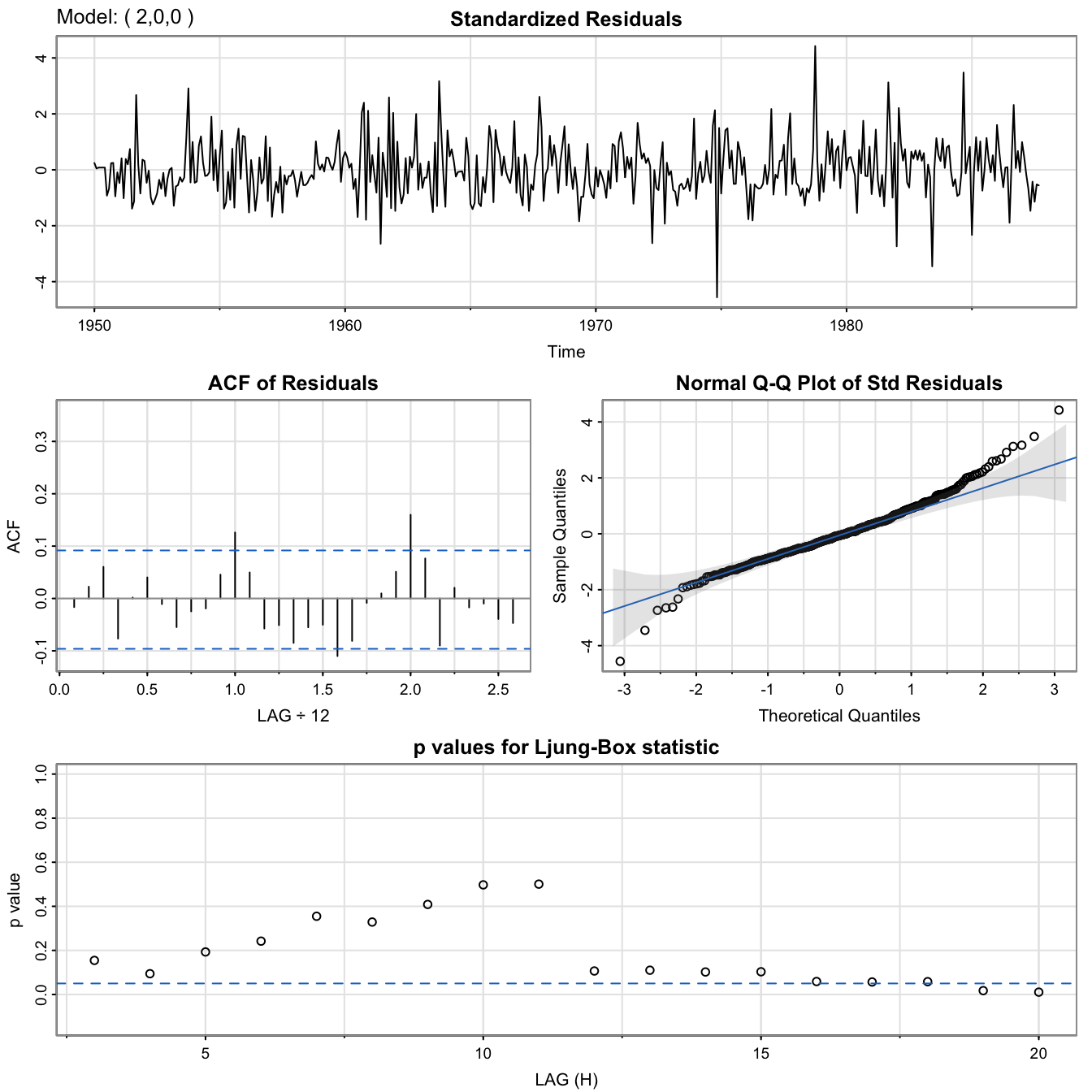
Diagnostics #
Guiding principle: if we have a good fit, the residuals should be (uncorrelated) white noise. This can be done in three ways:
- Residuals: If visual inspection of the residuals lets appear any pattern (trend or magnitude) then it can’t be white noise
- ACF and PACF: these should be within their confidence intervals with appropriate frequency (95%)
- More formally, one can test for white noise with the Ljung-Box portmanteau test. This test considers the dimension of the models (the number of parameters), and tests whether correlations are 0 at all lags, and displays
\(p\)-values. High\(p\)-values mean we cannot reject the (null) hypothesis of white noise (which is what we want).
In Base R , those three diagnostics are output when running the R function tsdiag(fit) where fit is where we stored our estimation from the function arima (but this function has errors!).
Better still, use the fitting function sarima(rec,2,0,0) of astsa.
tsdiag(rec.arima0)
[note no output in the console]
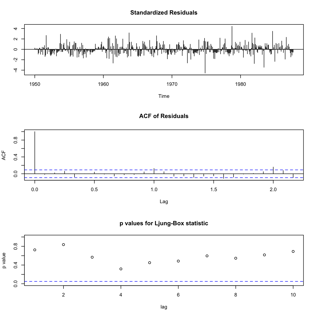
RecSARIMAdiag <- sarima(rec, 2, 0, 0)
## initial  value 3.332380
## iter   2 value 3.251366
## iter   3 value 2.564654
## iter   4 value 2.430141
## iter   5 value 2.258212
## iter   6 value 2.253343
## iter   7 value 2.248346
## iter   8 value 2.248345
## iter   9 value 2.248345
## iter  10 value 2.248341
## iter  11 value 2.248332
## iter  12 value 2.248331
## iter  13 value 2.248330
## iter  13 value 2.248330
## iter  13 value 2.248330
## final  value 2.248330
## converged
## initial  value 2.248862
## iter   2 value 2.248857
## iter   3 value 2.248855
## iter   4 value 2.248855
## iter   5 value 2.248854
## iter   6 value 2.248854
## iter   7 value 2.248854
## iter   8 value 2.248854
## iter   9 value 2.248853
## iter  10 value 2.248853
## iter  10 value 2.248853
## iter  10 value 2.248853
## final  value 2.248853
## converged
## <><><><><><><><><><><><><><>
##
## Coefficients:
##       Estimate     SE  t.value p.value
## ar1     1.3512 0.0416  32.4933       0
## ar2    -0.4612 0.0417 -11.0687       0
## xmean  61.8585 4.0039  15.4494       0
##
## sigma^2 estimated as 89.33436 on 450 degrees of freedom
##
## AIC = 7.353244  AICc = 7.353362  BIC = 7.389587
##
RecSARIMAdiag$fit
##
## Call:
## arima(x = xdata, order = c(p, d, q), seasonal = list(order = c(P, D, Q), period = S),
##     xreg = xmean, include.mean = FALSE, transform.pars = trans, fixed = fixed,
##     optim.control = list(trace = trc, REPORT = 1, reltol = tol))
##
## Coefficients:
##          ar1      ar2    xmean
##       1.3512  -0.4612  61.8585
## s.e.  0.0416   0.0417   4.0039
##
## sigma^2 estimated as 89.33:  log likelihood = -1661.51,  aic = 3331.02
RecSARIMAdiag$ICs
##      AIC     AICc      BIC
## 7.353244 7.353362 7.389587
Overfitting caveat #
- If we choose an order that is too high, the unnecessary parameters will be insignificant, but this reduces the efficiency of the parameters that are significant. This might look like a better fit, but might lead to bad forecasts. Hence, this should be avoided.
- This can be used as a diagnostic though: if we increment the order and we get similar parameter estimates, then the smaller (original) model should have the appropriate order.
Although generally not well-known, it is an obvious fact to seasoned modellers that extrapolating overfitted models is almost guaranteed to lead to aberrant results.
Example: Overfitting caveat #
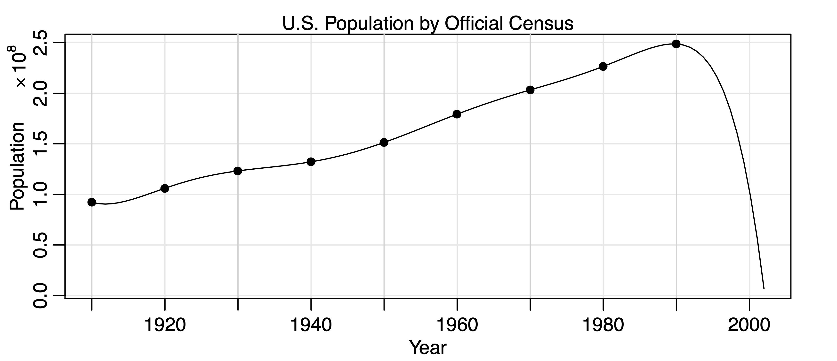
- shows the U.S. population by official census, every ten years from 1910 to 1990, as points. If we use these nine observations to predict the future population, we can use an eight-degree polynomial so the fit to the nine observations is perfect.
- The model predicts that the population of the United States will be close to zero in the year 2000, and will cross zero sometime
in the year 2002!
When seasonality is involved #
The process described above is applied by analogy when some seasonality is present in the residuals:
- Of course, the first step is to include a seasonal component in the trend if appropriate (such as with
\(\sin\)and\(\cos\)functions). - The series is then “in-season” and “out-of-season” differenced to lead to stationarity (if needed).
- Peaks in the ACF and PACF are then analysed with the tables presented at the beginning of this section, and eliminated with an appropriate
\(ARIMA(p,d,q)\times(P,D,Q)_s\)model. - Goodness-of-fit is assessed as usual by examining the whiteness of the residuals
(e.g., this can be done thanks to the diagnostics ofsarima)
Example: Air Passengers #
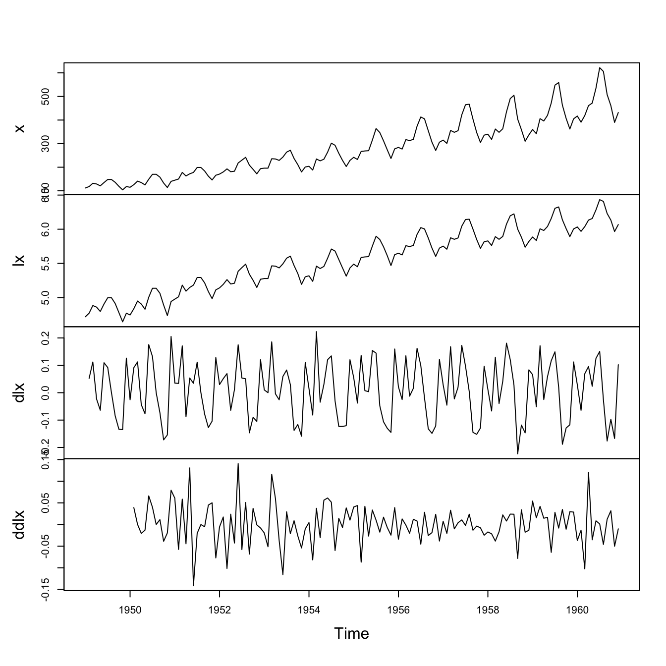
Remember the steps 1.-2. performed in the previous module:
x <- AirPassengers
lx <- log(x)
dlx <- diff(lx)
ddlx <- diff(dlx, 12)
plot.ts(cbind(x, lx, dlx, ddlx), main = "")
This corresponds to step 2 above, and had led to residuals that look reasonably stationary.
We now need to choose a model for them.
acf2(ddlx, 50)
##       [,1]  [,2]  [,3]  [,4] [,5] [,6]  [,7]  [,8] [,9] [,10] [,11]
## ACF  -0.34  0.11 -0.20  0.02 0.06 0.03 -0.06  0.00 0.18 -0.08  0.06
## PACF -0.34 -0.01 -0.19 -0.13 0.03 0.03 -0.06 -0.02 0.23  0.04  0.05
##      [,12] [,13] [,14] [,15] [,16] [,17] [,18] [,19] [,20] [,21]
## ACF  -0.39  0.15 -0.06  0.15 -0.14  0.07  0.02 -0.01 -0.12  0.04
## PACF -0.34 -0.11 -0.08 -0.02 -0.14  0.03  0.11 -0.01 -0.17  0.13
##      [,22] [,23] [,24] [,25] [,26] [,27] [,28] [,29] [,30] [,31]
## ACF  -0.09  0.22 -0.02  -0.1  0.05 -0.03  0.05 -0.02 -0.05 -0.05
## PACF -0.07  0.14 -0.07  -0.1 -0.01  0.04 -0.09  0.05  0.00 -0.10
##      [,32] [,33] [,34] [,35] [,36] [,37] [,38] [,39] [,40] [,41]
## ACF   0.20 -0.12  0.08 -0.15 -0.01  0.05  0.03 -0.02 -0.03 -0.07
## PACF -0.02  0.01 -0.02  0.02 -0.16 -0.03  0.01  0.05 -0.08 -0.17
##      [,42] [,43] [,44] [,45] [,46] [,47] [,48] [,49] [,50]
## ACF   0.10 -0.09  0.03 -0.04 -0.04  0.11 -0.05  0.11 -0.02
## PACF  0.07 -0.10 -0.06 -0.03 -0.12 -0.01 -0.05  0.09  0.13
Seasonal component:
- At the seasons, the ACF appears to be cutting off at lag
\(1s\)\((s=12)\) - PACF appears to be tailing off at lags
\(1s, 2s, 3s, 4s, \ldots\). \(\alert{\Longrightarrow SMA(1)}\),\(P=0\),\(Q=1\), in the season\(s=12\)
Non-Seasonal component:
- We inspect the ACF and PACF at lower lags.
- Both appear to be tailing off, which suggests ARMA within the seasons, say with
\(p=q=1\). \(\alert{\Longrightarrow ARMA(1,1)}\)
Thus, we will first try an \(ARIMA(1,1,1)\times(0,1,1)_{12}\)} on the logged data:
AirPassFit1 <- sarima(lx, 1, 1, 1, 0, 1, 1, 12)
AirPassFit1$fit
##
## Call:
## arima(x = xdata, order = c(p, d, q), seasonal = list(order = c(P, D, Q), period = S),
##     include.mean = !no.constant, transform.pars = trans, fixed = fixed, optim.control = list(trace = trc,
##         REPORT = 1, reltol = tol))
##
## Coefficients:
##          ar1      ma1     sma1
##       0.1960  -0.5784  -0.5643
## s.e.  0.2475   0.2132   0.0747
##
## sigma^2 estimated as 0.001341:  log likelihood = 244.95,  aic = -481.9
The AR parameter is not significant, so we try dropping one parameter from the within seasons part. We will try
AirPassFit2 <- sarima(lx, 0, 1, 1, 0, 1, 1, 12) # ARIMA(0,1,1)x(0,1,1)_12
AirPassFit3 <- sarima(lx, 1, 1, 0, 0, 1, 1, 12) # ARIMA(1,1,0)x(0,1,1)_12
AirPassFit2$fit
...
## Coefficients:
##           ma1     sma1
##       -0.4018  -0.5569
## s.e.   0.0896   0.0731
##
## sigma^2 estimated as 0.001348:  log likelihood = 244.7,  aic = -483.4
...
AirPassFit3$fit
...
## Coefficients:
##           ar1     sma1
##       -0.3395  -0.5619
## s.e.   0.0822   0.0748
##
## sigma^2 estimated as 0.001367:  log likelihood = 243.74,  aic = -481.49
...
AirPassFit2$ICs
##       AIC      AICc       BIC
## -3.690069 -3.689354 -3.624225
AirPassFit3$ICs
##       AIC      AICc       BIC
## -3.675493 -3.674777 -3.609649
All information criteria prefer the \(ARIMA(0,1,1)\times(0,1,1)_{12}\) model, which is displayed next.
AirPassFit2 <- sarima(lx, 0, 1, 1, 0, 1, 1, 12) # ARIMA(0,1,1)x(0,1,1)_12
Except for 1-2 outliers, the model fits well.
Checking whether we should have \(P=1\)?
#
AirPassFit4 <- sarima(lx, 0, 1, 1, 1, 1, 1, 12) # ARIMA(0,1,1)x(1,1,1)_12
AirPassFit2$ICs
##       AIC      AICc       BIC
## -3.690069 -3.689354 -3.624225
AirPassFit4$ICs
##       AIC      AICc       BIC
## -3.678726 -3.677284 -3.590934
All information criteria prefer the \(ARIMA(0,1,1)\times(0,1,1)_{12}\) model again.
AirPassFit4 <- sarima(lx, 0, 1, 1, 1, 1, 1, 12) # ARIMA(0,1,1)x(1,1,1)_12
Complete case study: GNP data #
plot(gnp, main = "Quarterly U.S. GNP from 1947(1) to 2002(3)")
GNP data seems to have exponential growth,
so a log transformation might be appropriate.
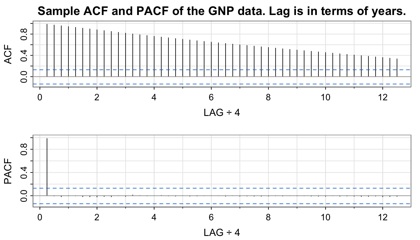
acf2(gnp, 50, main = "Sample ACF and PACF of the GNP data. Lag is in terms of years.")
...
##      [,1] [,2]  [,3] [,4] [,5]  [,6]  [,7]  [,8]  [,9] [,10] [,11]
## ACF  0.99 0.97  0.96 0.94 0.93  0.91  0.90  0.88  0.87  0.85  0.83
## PACF 0.99 0.00 -0.02 0.00 0.00 -0.02 -0.02 -0.02 -0.01 -0.02  0.00
...
Slow decay of ACF \(\rightarrow\) differencing may be appropriate.
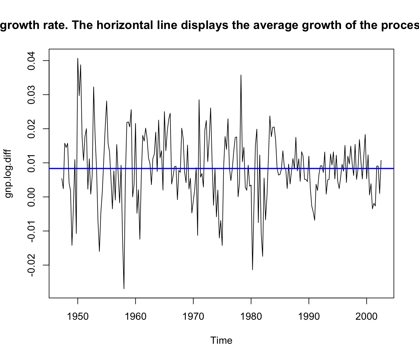
Making those two modifications leads to
gnp.log.diff <- diff(log(gnp))  # growth rate plot(gnpgr)
ts.plot(gnp.log.diff, main = "U.S. GNP quarterly growth rate. The horizontal line displays the average growth of the process, which is close to 1%.")
abline(mean(gnp.log.diff), 0, col = "blue", lwd = 2)
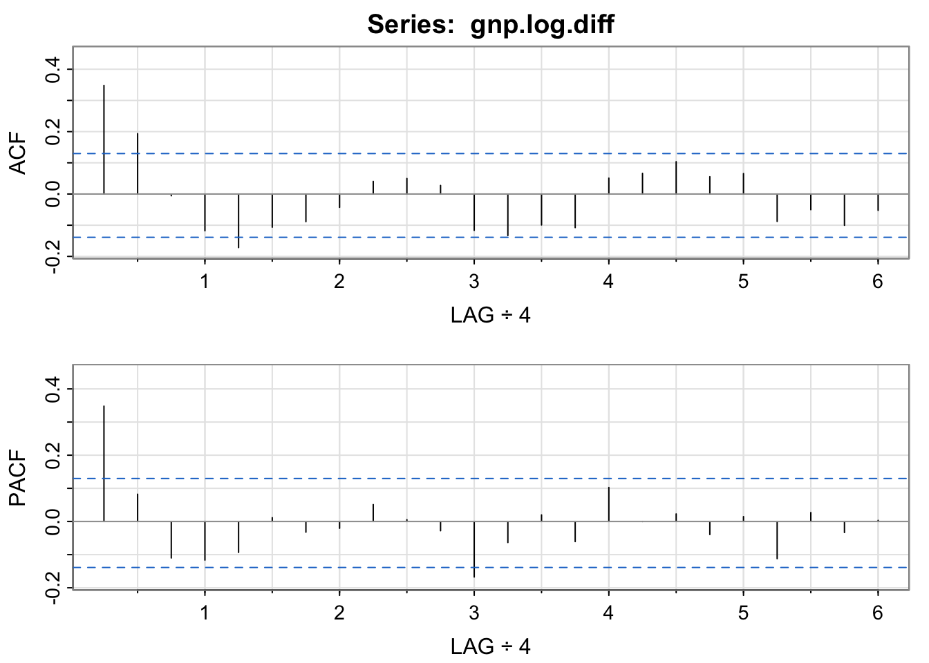
acf2(gnp.log.diff, 24)
...
##      [,1] [,2]  [,3]  [,4]  [,5]  [,6]  [,7]  [,8] [,9] [,10] [,11]
## ACF  0.35 0.19 -0.01 -0.12 -0.17 -0.11 -0.09 -0.04 0.04  0.05  0.03
## PACF 0.35 0.08 -0.11 -0.12 -0.09  0.01 -0.03 -0.02 0.05  0.01 -0.03
...
GNP data: \(MA(2)\) fit
#
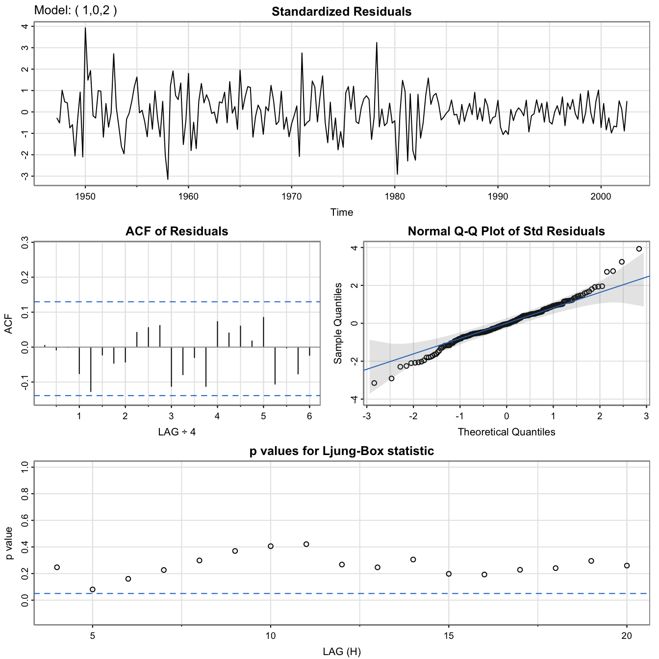
GNP.MA2 <- sarima(gnp.log.diff, 0, 0, 2) # MA(2)
GNP.MA2$fit
##
## Call:
## arima(x = xdata, order = c(p, d, q), seasonal = list(order = c(P, D, Q), period = S),
##     xreg = xmean, include.mean = FALSE, transform.pars = trans, fixed = fixed,
##     optim.control = list(trace = trc, REPORT = 1, reltol = tol))
##
## Coefficients:
##          ma1     ma2   xmean
##       0.3028  0.2035  0.0083
## s.e.  0.0654  0.0644  0.0010
##
## sigma^2 estimated as 8.919e-05:  log likelihood = 719.96,  aic = -1431.93
GNP.MA2$ICs
##       AIC      AICc       BIC
## -6.450133 -6.449637 -6.388823

GNP data: \(AR(1)\) fit
#
GNP.AR1 <- sarima(gnp.log.diff, 1, 0, 0) # AR(1)
GNP.AR1$fit
##
## Call:
## arima(x = xdata, order = c(p, d, q), seasonal = list(order = c(P, D, Q), period = S),
##     xreg = xmean, include.mean = FALSE, transform.pars = trans, fixed = fixed,
##     optim.control = list(trace = trc, REPORT = 1, reltol = tol))
##
## Coefficients:
##          ar1   xmean
##       0.3467  0.0083
## s.e.  0.0627  0.0010
##
## sigma^2 estimated as 9.03e-05:  log likelihood = 718.61,  aic = -1431.22
GNP.AR1$ICs
##       AIC      AICc       BIC
## -6.446940 -6.446693 -6.400958

GNP data: \(ARMA(1,2)\) fit
#
GNP.ARMA <- sarima(gnp.log.diff, 1, 0, 2) # ARMA(1,2)
GNP.ARMA$fit
##
## Call:
## arima(x = xdata, order = c(p, d, q), seasonal = list(order = c(P, D, Q), period = S),
##     xreg = xmean, include.mean = FALSE, transform.pars = trans, fixed = fixed,
##     optim.control = list(trace = trc, REPORT = 1, reltol = tol))
##
## Coefficients:
##          ar1     ma1     ma2   xmean
##       0.2407  0.0761  0.1623  0.0083
## s.e.  0.2066  0.2026  0.0851  0.0010
##
## sigma^2 estimated as 8.877e-05:  log likelihood = 720.47,  aic = -1430.95
GNP.ARMA$ICs
##       AIC      AICc       BIC
## -6.445712 -6.444882 -6.369075
GNP data: Comparison #
Note fitted models are
- MA(2):
$$\hat{x}_t=0.008_{(0.001)}+0.303_{(0.065)}\hat{w}_{t-1}+0.204_{(0.064)}\hat{w}_{t-2}+\hat{w}_t,$$where\(\hat{\sigma}_w=0.0094\). - AR(1):
$$\hat{x}_t=0.008_{(0.001)}(1-0.347)+0.347_{(0.063)}\hat{x}_{t-1}+\hat{w}_t,$$where\(\hat{\sigma}_w=0.0095\).
- In fact, both models are nearly the same. This is because the AR model can be rewritten (ignoring the constant) as
$$x_t \approx 0.35 w_{t-1}+0.12 w_{t-2}+w_t,$$where the coefficients were obtained via
formatC(ARMAtoMA(ar = 0.35, ma = 0, 6), digits = 3)
## [1] "0.35"    "0.122"   "0.0429"  "0.015"   "0.00525" "0.00184"
GNP data: Model selection #
- Information criteria (the lower the better):
- AR(1):
$AIC: -6.446940$AICc: -6.446693$BIC: -6.400958 - MA(2):
$AIC: -6.450133$AICc: -6.449637$BIC: -6.388823 - ARMA(1,2):
$AIC: -6.445712$AICc: -6.444882$BIC: -6.369075
- AR(1):
- The AIC and AICc both prefer the MA(2) fit to AR(1)
- The BIC prefers the simpler AR(1) model to MA(2).
- It is often the case that the BIC will select a model of smaller order than the AIC or AICc. In either case, it is not unreasonable to retain the AR(1) because pure autoregressive models are easier to work with.
- Combining the two to
\(ARMA(1,2)\)leads to poorer scores.
Side comment: compare with ARIMA(1,1,2) on log(GNP) #
GNP.MA2 <- sarima(log(gnp), 1, 1, 2) # ARIMA(1,1,2)
GNP.MA2$fit
##
## Call:
## arima(x = xdata, order = c(p, d, q), seasonal = list(order = c(P, D, Q), period = S),
##     xreg = constant, transform.pars = trans, fixed = fixed, optim.control = list(trace = trc,
##         REPORT = 1, reltol = tol))
##
## Coefficients:
##          ar1     ma1     ma2  constant
##       0.2407  0.0761  0.1623    0.0083
## s.e.  0.2066  0.2026  0.0851    0.0010
##
## sigma^2 estimated as 8.877e-05:  log likelihood = 720.47,  aic = -1430.95
GNP.MA2$ICs
##       AIC      AICc       BIC
## -6.445711 -6.444880 -6.369074

Appendix: Method of moments for \(AR(p)\) models
#
We seek to estimate \(\phi_1, \ldots, \phi_p\) in the \(AR(p)\) model
$$x_t=\phi_1 x_{t-1}+\cdots+\phi_p x_{t-p} + w_t.$$
A method of moments approach leads us back to the Yule-Walker equations
$$\begin{array}{rcl} \gamma(h) &=& \phi \gamma(h-1)+\cdots + \phi_p \gamma(h-p), \quad h=1,2,\ldots, p\\ \sigma_w^2 &=& \gamma(0)-\phi_1 \gamma(1)-\cdots-\phi_p \gamma(p). \end{array}$$
In matrix notation, these become
$$\Gamma_p \phi = \gamma_p\quad\text{and}\quad\sigma_w^2=\gamma(0)-\phi'\gamma_p.$$
where
$$\Gamma_p=\{\gamma(k-j)\}_{j,k=1}^p$$
is a \(p\times p\) matrix.
Using the method of moments, we replace \(\gamma(h)\) by \(\hat{\gamma}(h)\) and solve
$$\hat{\phi}=\hat{\Gamma}_p^{-1} \hat{\gamma}_p, \quad \hat{\sigma}^2_w=\hat{\gamma}(0)-\hat{\gamma}'_p\hat{\Gamma}_p^{-1}\hat{\gamma}_p.$$
These are called the Yule-Walker estimators. Equivalently
$$\hat{\phi}=\hat{\Gamma}_p^{-1} \hat{\rho}_p, \quad \hat{\sigma}^2_w=\hat{\gamma}(0)\left[ 1-\hat{\rho}'_p\hat{R}_p^{-1}\hat{\rho}_p\right],$$
$$\text{where }\hat{R}_p=\{\hat{\rho}(k-j)\}_{j,k=1}^p \text{ is a }p\times p\text{ matrix.}$$
- For
\(AR(p)\)models, if the sample size is large, the Yule-Walker estimators are approximately normally distributed, and\(\hat{\sigma}_w^2\)is close to the true value of\(\sigma_w^2\). - The Yule-Walker estimators are essentially least square estimators, which work well on AR models because they are linear. MA (and ARMA) processes are nonlinear in the parameters, and will fare badly with the Yule-Walker estimators.
Example: Recruitment series #
Yule-Walker estimators are implemented in R as follows:
rec.yw <- ar.yw(rec, order = 2)
rec.yw$x.mean  #  (mean estimate)
## [1] 62.26278
rec.yw$ar  # (coefficient estimates)
## [1]  1.3315874 -0.4445447
sqrt(diag(rec.yw$asy.var.coef))  # (standard errors)
## [1] 0.04222637 0.04222637
rec.yw$var.pred  # (error variance estimate)
## [1] 94.79912
The fit is then displayed as follows:
ts.plot(rec, main = "Results of fit using the Yule-Walker estimators")
lines(rec[1:length(rec)] - rec.yw$resid, col = "blue", lwd = 1)
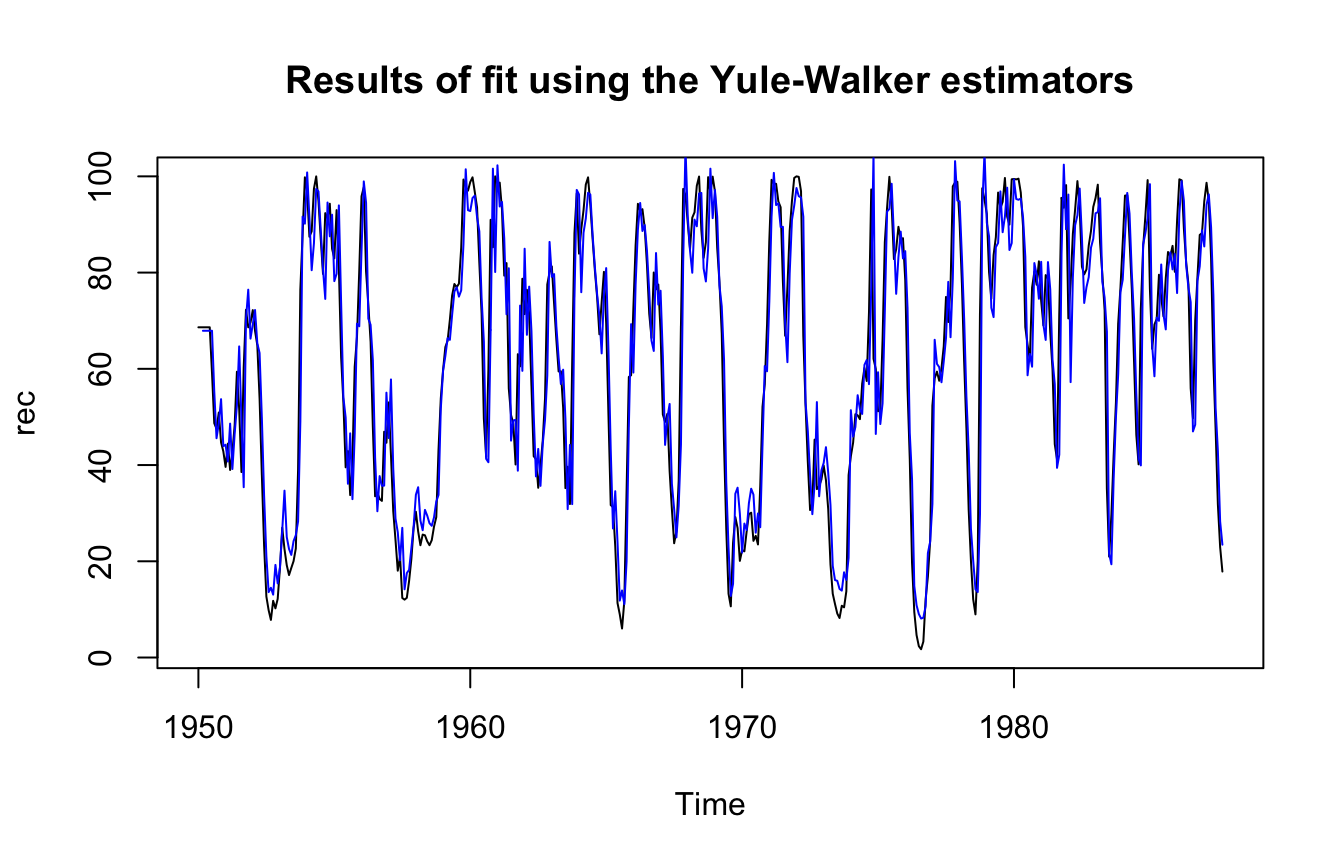
The estimators obtained are nearly identical to the MLE ones (although MLE has lower variance as expected). It can be shown that this will typically be the case for AR models.
\(\adv\) Comparison of estimation techniques via residuals of rec
#
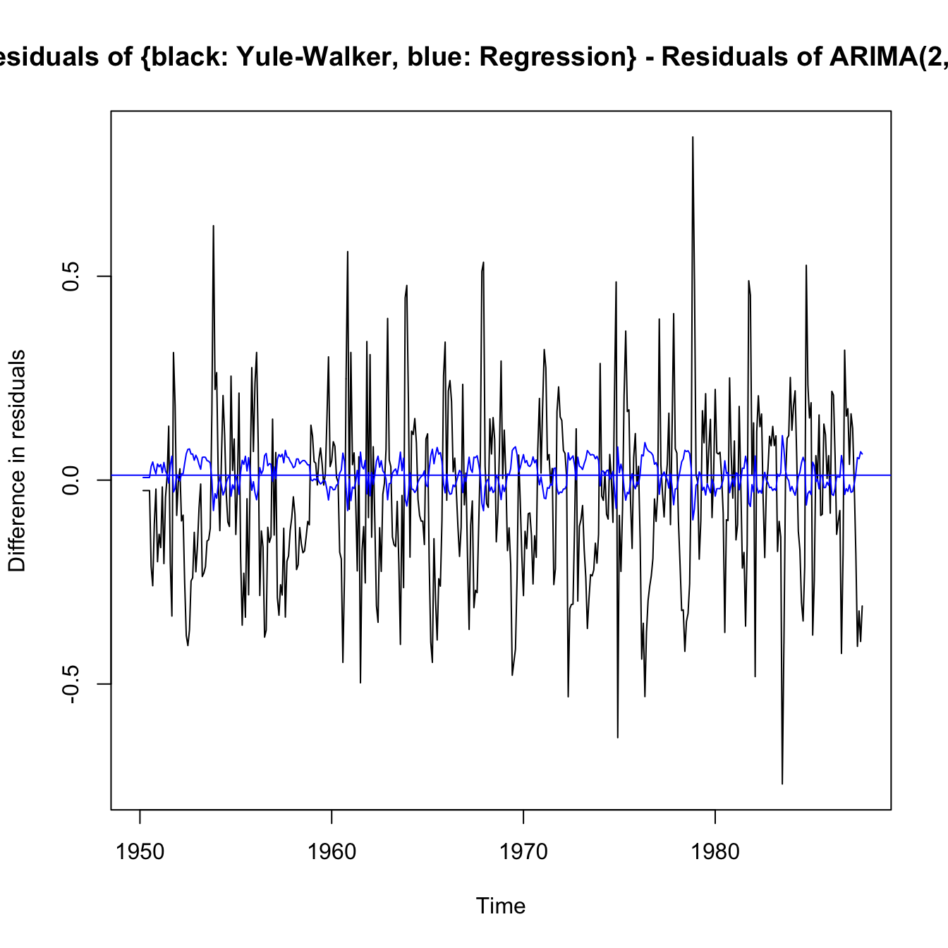
ts.plot(rec.yw$resid - rec.arima$fit$residuals, ylab = "Difference in residuals",
  main = "Residuals of {black: Yule-Walker, blue: Regression} - Residuals of ARIMA(2,0,0) fit")
abline(a = mean((rec.yw$resid[3:length(rec)] - rec.arima$fit$residuals[length(rec)])^1),
  0, col = "black")
lines(regr$resid - rec.arima$fit$residuals, col = "blue")
abline(a = mean((regr$resid[3:length(rec)] - rec.arima$fit$residuals[3:length(rec)])^1),
  0, col = "blue")
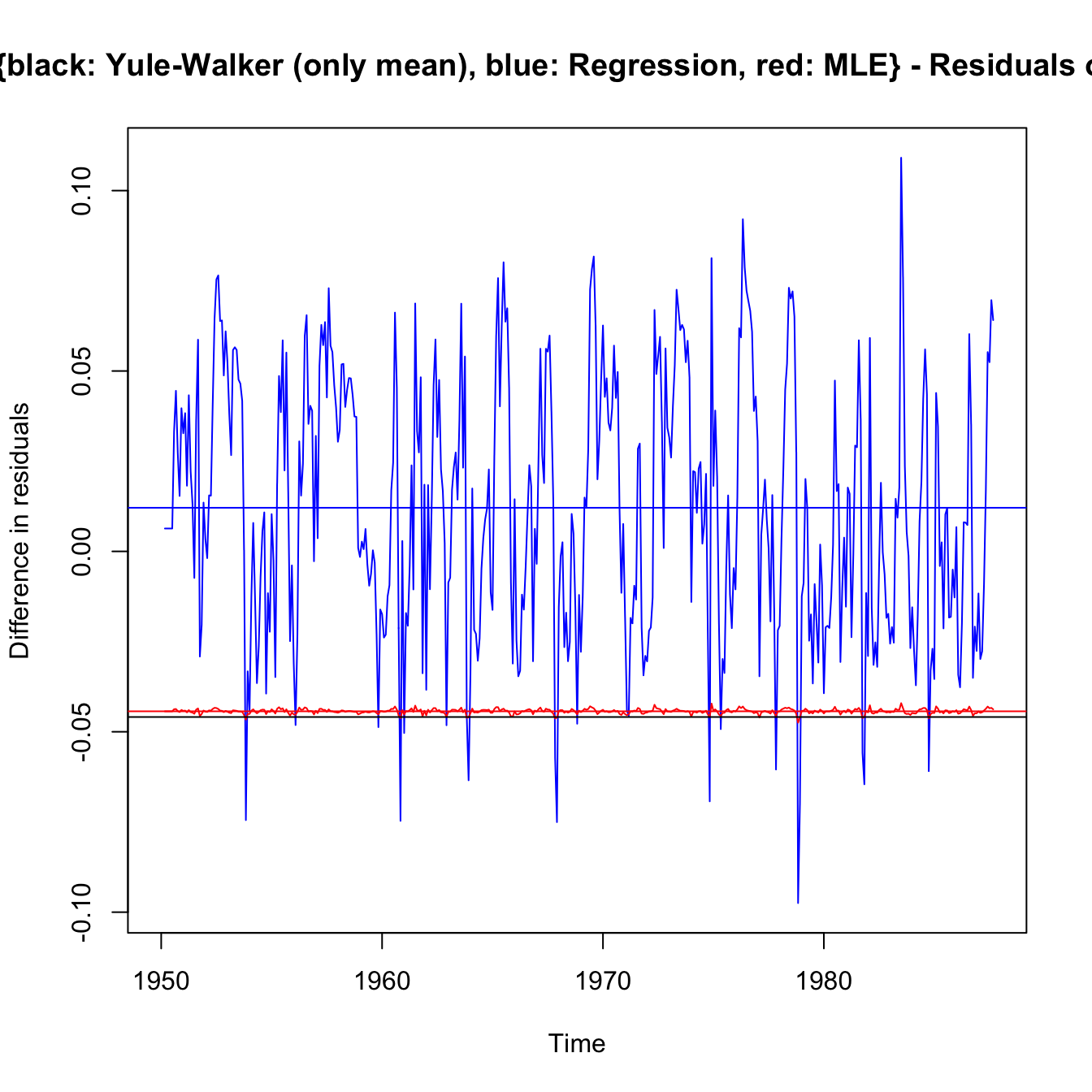
ts.plot(regr$resid - rec.arima$fit$residuals, col = "blue", ylab = "Difference in residuals",
  main = "Residuals of {black: Yule-Walker (only mean), blue: Regression, red: MLE} - Residuals of ARIMA(2,0,0) fit")
abline(a = mean((regr$resid[3:length(rec)] - rec.arima$fit$residuals[3:length(rec)])^1),
  0, col = "blue")
lines(rec.mle$resid - rec.arima$fit$residuals, col = "red")
abline(a = mean((rec.mle$resid[3:length(rec)] - rec.arima$fit$residuals[3:length(rec)])),
  0, col = "red")
# lines(rec.yw$resid-rec.arima$fit$residuals,col='black')
abline(a = mean((rec.yw$resid[3:length(rec)] - rec.arima$fit$residuals[3:length(rec)])^1),
  0, col = "black")
Model residuals \(\equiv\) innovations \(\alert{\hat{e}}\) |
Mean | \(\Delta\) to arima |
\(\sum \hat{e}^2\) |
|---|---|---|---|
regr$resid[3:length(rec)] |
0.000 | -0.020 | 40343 |
rec.yw$resid[3:length(rec)] |
-0.021 | -0.041 | 40369 |
rec.mle$resid[3:length(rec)] |
-.020 | -0.040 | 40344 |
rec.arima$fit$residuals[3:length(rec)] |
0.020 | - | 404344 |
- Yule-Walker and MLE are very close (location) as pointed out earlier.
- Yule-Walker is focussed on moments irrespective of residuals, so it is the poorest in terms of least squares.
- As compared to Yule-Walker and MLE, the
arimamethodology sacrifices some Least Square performance in favour of a better fit (mean of residuals is closer to 0). Flatness of MLE (in red) suggestsarimais a shifted MLE. It seems to be the best compromise. - The regression is pure least squares, and minimises them, and has 0 mean residuals. However, it can’t be the preferred model as it ignores the fact that the model is autoregressive, and is not regressed on an independent, assumed known and independent, series. Forecasts (and their standard errors) should not be trusted.
(see next slide for code that generated numbers)
mean((regr$resid[3:length(rec)] - rec.arima$fit$residuals[3:length(rec)])^1)
## [1] 0.01208978
mean((rec.yw$resid[3:length(rec)] - rec.arima$fit$residuals[3:length(rec)])^1)
## [1] -0.04591007
mean((rec.mle$resid[3:length(rec)] - rec.arima$fit$residuals[3:length(rec)])^1)
## [1] -0.04432752
mean(regr$resid[3:length(rec)]^1)
## [1] -3.17507e-13
mean(rec.yw$resid[3:length(rec)]^1)
## [1] -0.05799985
mean(rec.mle$resid[3:length(rec)]^1)
## [1] -0.05641729
mean(rec.arima$fit$residuals[3:length(rec)]^1)
## [1] -0.01208978
sum(regr$resid[3:length(rec)]^2)
## [1] 40462.39
sum(rec.yw$resid[3:length(rec)]^2)
## [1] 40491.55
sum(rec.mle$resid[3:length(rec)]^2)
## [1] 40464.39
sum(rec.arima$fit$residuals[3:length(rec)]^2)
## [1] 40463.03
Forecasting #
Introduction #
- In forecasting, the goal is to predict future values of a time series,
\(x_{n+m}\),\(m = 1, 2,\ldots\), based on the data collected to the present,\(x_{1:n} = \{x_1, x_2,\ldots, x_n\}\). - We assume here that
\(x_t\)is stationary and the model parameters are known. - The problem of forecasting when the model parameters are unknown is more complicated. We mostly focus on performing predictions using R (which allows for that fact appropriately), rather than the deep technicalities of it (which are outside scope of this course).
Best Linear Predictors (BLPs) #
We will restrict our attention to predictors that are linear functions of the data, that is, predictors of the form
$$x_{n+m}^n = \alpha_0 + \sum_{k=1}^n \alpha_k x_k,$$
where \(\alpha_0,\alpha_1,\ldots, \alpha_n\) are real numbers. These are called Best Linear Predictors (BLPs).
Note:
- In fact the
\(\alpha\)’s depend on\(m\)too, but that is not reflected in the notation. - Such estimators depend only on the second-order moments of the process, which are easy to estimate from the data.
- Most actuarial credibility estimators belong to the family of BLPs (Bühlmann, Bühlmann-Straub,
\(\ldots\))
Best Linear Prediction for Stationary Processes #
Given data \(x_1,\ldots,x_n\), the best linear predictor
$$x_{n+m}^n = \alpha_0 + \sum_{k=1}^n \alpha_k x_k$$
of \(x_{n+m}\) for \(m\ge 1\) is found by solving
$$E\left[ (x_{n+m}-x_{n+m}^n)x_k\right]=0,\quad k=0,1,\ldots,n,$$
where \(x_0=1\), for \(\alpha_0, \alpha_1, \ldots, \alpha_n\).
- The
\(n+1\)equations specified above are called the prediction equations, and they are used to solve for the coefficients\(\{\alpha_0,\alpha_1,\ldots,\alpha_n\}\). - This results stems from minimising least squares.
If \(E[x_t]=\mu\), the first equation \((k=0)\) implies
$$E[x_{n+m}^n]=E[x_{n+m}]=\mu.$$
Thus, taking expectation of the BLP leads to
$$\mu=\alpha_0 +\sum_{k=1}^n \alpha_k \mu\quad \text{ or }\quad \alpha_0=\mu\left( 1-\sum_{k=1}^n \alpha_k \right).$$
Hence, the form of the BLP is
$$x_{n+m}^n = \mu + \sum_{k=1}^n \alpha_k (x_k-\mu)$$
Henceforth, we will assume that \(\mu=0\Longleftrightarrow \alpha_0=0\), without loss of generality (as long as parameters are assumed known).
One-step-ahead prediction #
- Given
\(x_{1:n} = \{x_1, x_2,\ldots, x_n\}\)we wish to forecast the time series\(x_{n+1}\)value at the next point in time\(n+1\). - The BLP of
\(x_{n+1}\)is of the form$$x_{n+1}^n = \phi_{n1} x_n + \phi_{n2} x_{n-1}+\cdots + \phi_{nn} x_1,$$where we now display the dependence of the coefficients on\(n\). - In this case,
\(\alpha_k\)is\(\phi_{n,n+1-k}\)for\(k=1,\ldots, n\). - Using the BLP result above, the coefficients
\(\{\phi_{n1},\phi_{n2},\ldots,\phi_{nn}\}\)satisfy$$\sum_{j=1}^n \phi_{nj}\gamma(k-j)=\gamma(k)\text{ for }k=1,\ldots,n\quad\text{ or } \Gamma_n \phi_n =\gamma_n,$$where\(\Gamma_n=\{\gamma(k-j)\}_{j,k=1}^n\)is an\(n\times n\)matrix,\(\phi_n=(\phi_{n1},\ldots,\phi_{nn})'\), and where\(\gamma_n=(\gamma(1),\ldots,\gamma(n))'\).
[Note that these correspond to the Yule-Walker equations.]
- The matrix
\(\Gamma_n\)is nonnegative definite (in fact guaranteed positive definite for ARMA models). We have then$$\phi_n=\Gamma_n^{-1} \gamma_n.$$ - The one-step-ahead forecast is then
$$x_{n+1}^n=\phi_n' x,\quad x=(x_n,x_{n-1},\ldots,x_1)'.$$ - The mean square one-step-ahead prediction error is
$$P_{n+1}^n = E\left[(x_{n+1}-x_{n+1}^n)^2\right]=\gamma(0)-\gamma_n'\Gamma_n^{-1}\gamma_n.$$
\(\adv\) The Durbin-Levinson Algorithm
#
The prediction equations (and associated mean-square errors) of the one-step-ahead prediction can be found iteratively thanks to the Durbin-Levinson Algorithm:
- Initial values:
$$\phi_{00}=0, \quad P_1^0=\gamma(0).$$ - For all
\(n\ge 1\)the last\(\phi\)is:$$\phi_{nn}=\frac{\rho(n)-\sum_{k=1}^{n-1}\phi_{n-1,k}\rho(n-k)}{1-\sum_{k=1}^{n-1}\phi_{n-1,k}\rho(k)}.$$ - If
\(n\ge 2\), middle\(\phi\)’s are:$$\phi_{nk}=\phi_{n-1,k}-\phi_{nn}\phi_{n-1,n-k},\quad k=1,2,\ldots,n-1.$$ - For
\(n\ge 1\), the prediction error is$$P_{n+1}^n=P_{n}^{n-1}(1-\phi_{nn}^2)=\gamma(0)\prod_{j=0}^n\left[ 1-\phi_{jj}^2\right].$$
Concluding notes #
- The results shown above are provided to illustrate the process of forecasting. Students are not expected to be able to show the results.
- There are other algorithms for calculating one-step-ahead forecasts, such as the innovations algorithm (outside scope).
\(\adv\)The Durbin-Levinson Algorithm can be adapted to calculate the PACF iteratively.
Forecasting ARMA processes #
Introduction #
- The technical side of forecasting ARMA models can get involved.
- Throughout, we assume
\(x_t\)is a causal and invertible\(ARMA(p,q)\)process$$\phi(B)x_t=\theta(B)w_t,\text{ where }w_t\sim\text{ iid N}(0,\sigma_w^2).$$ - In the non-zero mean case
\(E[x_t]=\mu_x\), simply replace\(x_t\)with\(x_t-\mu_x\)in the model.
Two types of forecasts #
We consider two types of forecasts:
- The minimum mean square error predictor of
\(x_{n+m}\)based on the data\(\{x_n,\ldots,x_1\}\), defined as$$x_{n+m}^n=E\left[ x_{n+m}|x_n,x_{n-1},\ldots,x_1\right].$$ - The predictor of
\(x_{n+m}\)based on the infinite past, defined as$$\tilde{x}_{n+m}=E\left[ x_{n+m}|x_n,x_{n-1},\ldots,x_1,\alert{x_0,x_{-1},\ldots} \right].$$
Note:
- For ARMA models,
\(\tilde{x}_{n+m}\)is easier to calculate. - In general,
\(x_{n+m}^n\)and\(\tilde{x}_{n+m}\)are not the same. - The idea is that, for large samples,
\(\tilde{x}_{n+m}\)provides a good approximation to\(x_{n+m}^n\).
Forecasts for more than one step #
Write \(x_{n+m}\) in its invertible form:
$$w_{n+m}=\sum_{j=0}^\infty \pi_j x_{n+m-j}, \quad \pi_0=1.$$
Taking conditional expectations we have
$$0=\tilde{x}_{n+m}+\sum_{j=\alert{1}}^\infty \pi_j \tilde{x}_{n+m-j}.$$
Because \(E[x_t|x_n,x_{n-1},\ldots,x_0,x_{-1},\ldots]=x_t\) for \(t\le n\) this can be rewritten as
$$\tilde{x}_{n+m}=-\sum_{j=1}^{\alert{m-1}} \pi_j \tilde{x}_{n+m-j}-\sum_{j=\alert{m}}^{\infty} \pi_j \alert{x}_{n+m-j}.$$
the second part of which belongs to the past.
Prediction is then accomplished recursively using
$$\tilde{x}_{n+m}=-\sum_{j=1}^{m-1} \pi_j \tilde{x}_{n+m-j}-\sum_{j=m}^{\infty} \pi_j x_{n+m-j},$$
starting with the one-step-ahead \((m=1)\), and then continuing for \(m=2,3,\ldots\).
This illustrates why it is easier to forecast with \(\tilde{x}_{n+m}\) Thanks to the infinite representation of \(x_t\) (if causal), extending the condition of the predictor \(x_{n+m}^n\) to infinite past allowed us the simple calculations above.
Mean-square prediction error is calculated next, but we need an intermediary result first - an expression for \(\tilde{x}_{n+m}\) in function of \(w\)’s (so we can calculate variance easily).
Write \(x_{n+m}\) in its causal form:
$$x_{n+m}=\sum_{j=0}^\infty \psi_j w_{n+m-j}, \quad \psi_0=1.$$
Taking conditional expectations we have
$$\tilde{x}_{n+m}=\sum_{j=0}^\infty \psi_j \tilde{w}_{n+m-j}=\sum_{j=\alert{m}}^\infty \psi_j \alert{w}_{n+m-j}$$
because
$$\tilde{w}_t = E[w_t|x_n,x_{n-1},\ldots,x_0,x_{-1},\ldots]=\left\{\begin{array}{lc} 0 & t>n \\ w_t & t\le n. \end{array}\right.$$
Mean-square prediction error can now be calculated thanks to
$$\tilde{x}_{n+m}=\sum_{j=m}^\infty \psi_j w_{n+m-j} \Longrightarrow x_{n+m}-\tilde{x}_{n+m}=\sum_{j=0}^{m-1}\psi_j w_{n+m-j},$$
and hence
$$P_{n+m}^n=E[(x_{n+m}-\tilde{x}_{n+m})^2]=\sigma_w^2\sum_{j=0}^{m-1}\psi_j^2.$$
Note that for a fixed sample size, \(n\), the prediction errors are correlated. That is, for time lag \(k\ge 1\),
$$ E\left[(x_{n+m}-\tilde{x}_{n+m})(x_{n+m+k}-\tilde{x}_{n+m+k})\right] = \sigma_w^2 \sum_{j=0}^{m-1} \psi_j \psi_{j+k}.$$
Predictions in practice #
- When
\(n\)is small the system of “prediction equations”$$E\left[ (x_{n+m}-x_{n+m}^n)x_k\right]=0,\quad k=0,1,\ldots,n,$$(where\(x_0=1\), for\(\alpha_0, \alpha_1, \ldots, \alpha_n\)) can be solved directly. - However, when
\(n\)is large one will want to use$$\tilde{x}_{n+m}=-\sum_{j=1}^{m-1} \pi_j \tilde{x}_{n+m-j}-\sum_{j=m}^{\infty} \pi_j x_{n+m-j}.$$This is correct “in theory”, but unfortunately, in practice we do not observe\(x_0, x_{-1},x_{-2},\ldots\), and only data\(x_1, x_2, \ldots,x_n\)are available. We then need to truncate the infinite sum in the RHS.
- The truncated predictor is then written as
$$\tilde{x}_{n+m}^{\alert{n}}=-\sum_{j=1}^{m-1} \pi_j \tilde{x}_{n+m-j}^{\alert{n}}-\sum_{j=m}^{\alert{n+m-1}} \pi_j x_{n+m-j},$$which is applied recursively as described above. - The mean square prediction error, in this case, is approximated using
\(P_{n+m}^n\)as before.
Truncated prediction for ARMA #
For \(ARMA(p,q)\) models, the truncated predictors for \(m=1,2,\ldots\) are
$$\tilde{x}_{n+m}^n=\phi_1\tilde{x}_{n+m-1}^n+\cdots+\phi_p\tilde{x}_{n+m-p}^n+\theta_1\tilde{w}_{n+m-1}^n+\cdots+\theta_q\tilde{w}_{n+m-q}^n,$$
where \(\tilde{x}_t^n=x_t\) for \(1\le t\le n\) and \(\tilde{x}_t^n=0\) for \(t\le 0\). The truncated prediction errors are given by
$$\tilde{w}_t^n=\left\{\begin{array}{lc} 0 & t\le 0 \text{ or }t>n \\ \phi(B)\tilde{x}_n^n-\theta_1\tilde{w}_{t-1}^n-\cdots-\theta_q \tilde{w}_{t-q}^n & 1\le t\le n. \end{array}\right.$$
(See Example 3.24 for an illustration). Note:
- For
\(AR(p)\)models with\(n>p\),$$\tilde{x}_{n+m}^n=\tilde{x}_{n+m}=x_{n+m}^n$$and there is no need for approximations. - The above approximation is required for
\(MA(q)\)and\(ARMA(p,q)\)models with\(q>0\).
Long-range forecasts #
- Consider forecasting an ARMA process with mean
\(\mu_x\). - Replacing
\(x_{n+m}\)with\(x_{n+m}-\mu_x\)in the causal representation above, and taking expectation in an analogous way implies that the\(m\)-step-ahead forecast can be written as$$\tilde{x}_{n+m}=\mu_x+\sum_{j=m}^\infty \psi_j w_{n+m-j}.$$ - Because the
\(\psi\)dampen to zero exponentially fast,$$\tilde{x}_{n+m}\rightarrow \mu_x \text{ exponentially fast as }m\rightarrow \infty.$$ - Moreover, the mean square prediction error
$$P_{n+m}^n\rightarrow \sigma_w^2 \sum_{j=0}^\infty \psi_j^2 = \gamma_x(0)=\sigma_x^2 \text{ exponentially fast as }m\rightarrow \infty.$$ - ARMA forecasts quickly settle to the mean with a constant prediction error as the forecast horizon,
\(m\), grows.
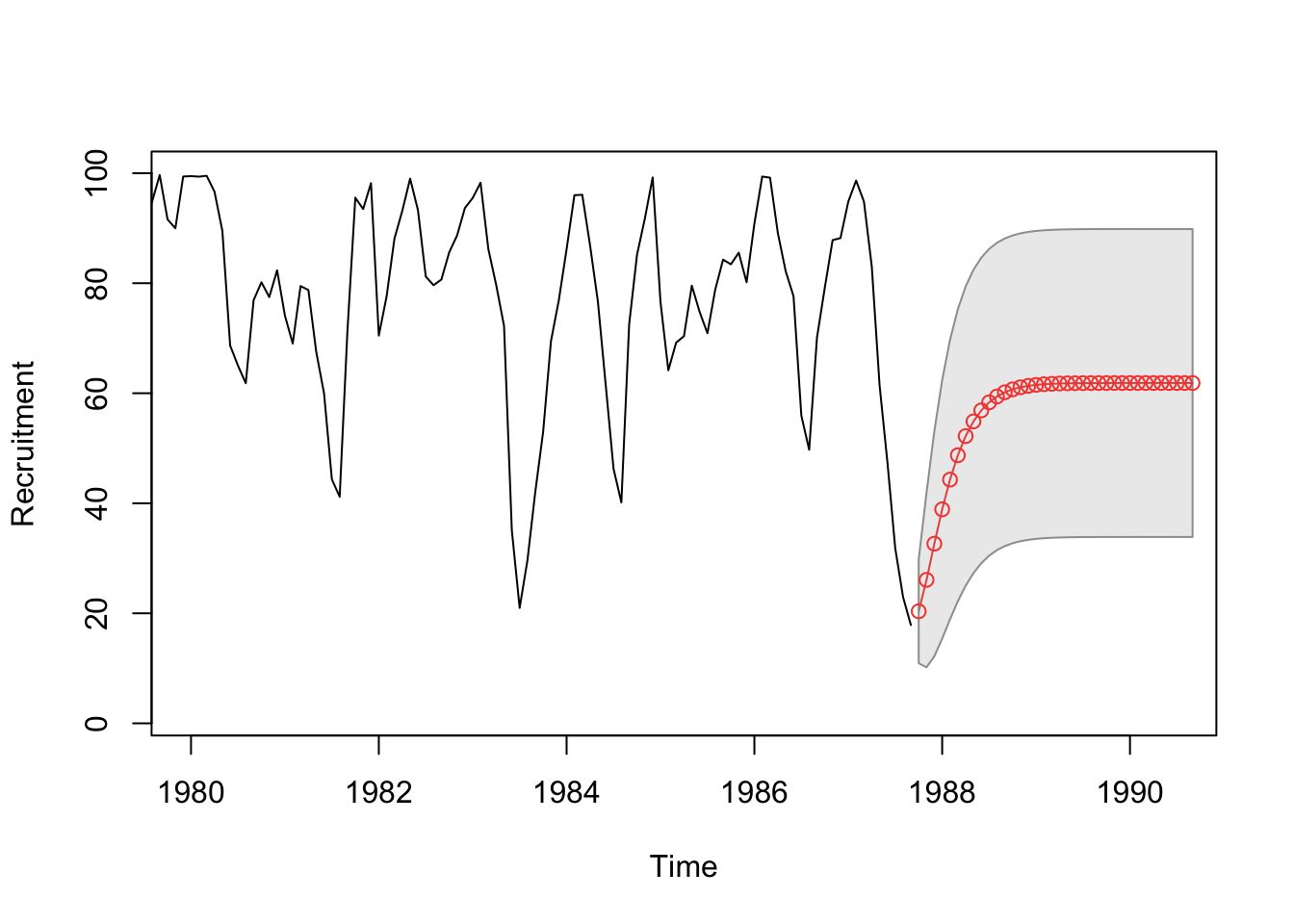
Example: Recruitment Series #
fore2 <- predict(rec.arima0, n.ahead = 36)
cbind(fore2$pred, fore2$se)
...
##          fore2$pred  fore2$se
## Oct 1987   20.36547  9.451686
## Nov 1987   26.08036 15.888378
## Dec 1987   32.65148 20.464325
## Jan 1988   38.89474 23.492457
## Feb 1988   44.30006 25.393693
## Mar 1988   48.72437 26.537088
## Apr 1988   52.20958 27.199368
## May 1988   54.87831 27.570234
## Jun 1988   56.87693 27.771616
## Jul 1988   58.34666 27.877923
## Aug 1988   59.41079 27.932597
## Sep 1988   60.17081 27.960042
## Oct 1988   60.70697 27.973508
## Nov 1988   61.08091 27.979974
## Dec 1988   61.33890 27.983014
...
ts.plot(rec, fore2$pred, col = 1:2, xlim = c(1980, 1990.5), ylab = "Recruitment")
U <- fore2$pred + fore2$se
L <- fore2$pred - fore2$se
xx <- c(time(U), rev(time(U)))
yy <- c(L, rev(U))
polygon(xx, yy, border = 8, col = gray(0.6, alpha = 0.2))
lines(fore2$pred, type = "p", col = 2)
Example: Air Passengers #
We forecast the model chosen in the previous section:
sarima.for(lx, 12, 0, 1, 1, 0, 1, 1, 12)
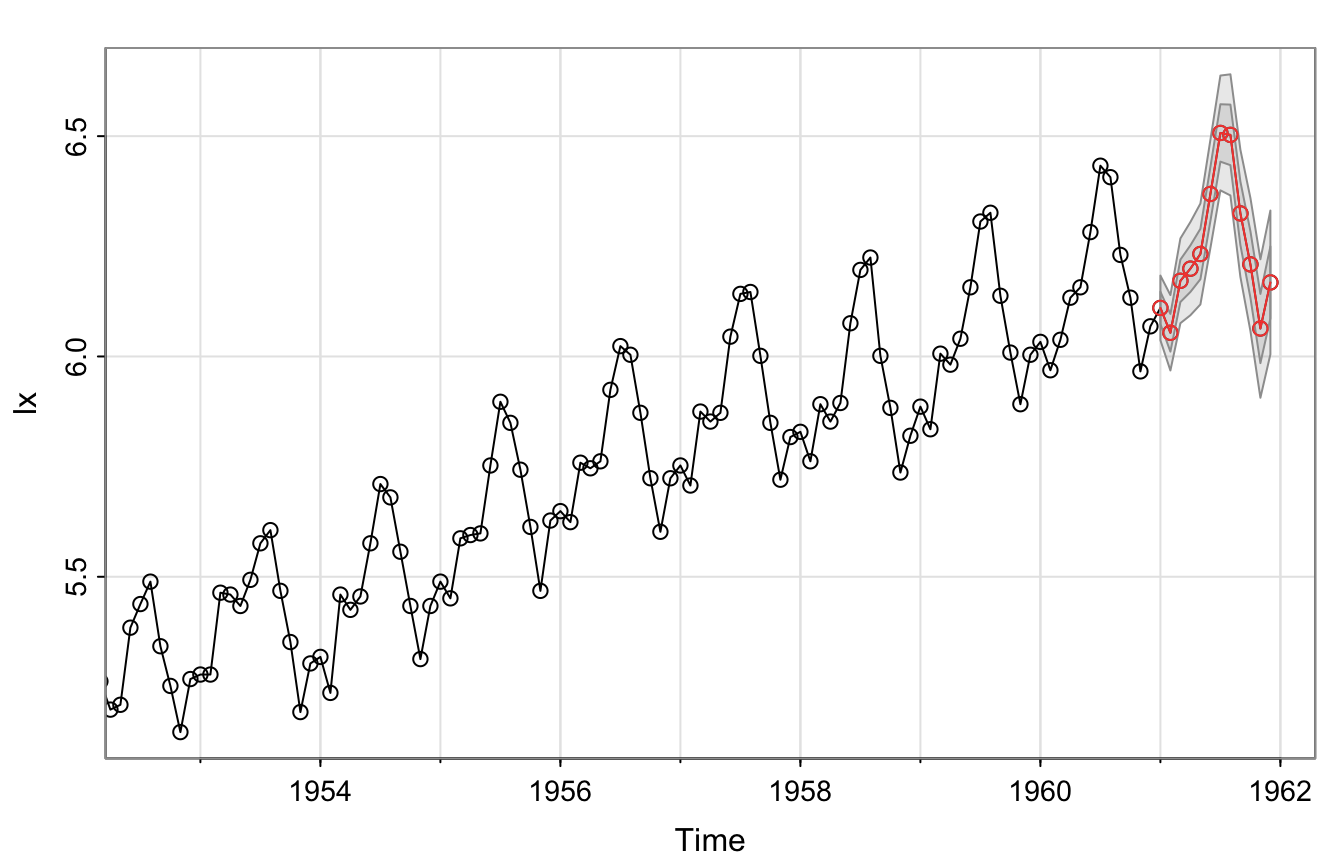
Including seasonality leads (apparently) to much higher precision.
References #
Shumway, Robert H., and David S. Stoffer. 2017. Time Series Analysis and Its Applications: With r Examples. Springer.