Dependence and multivariate modelling #
Introduction to Dependence #
Motivation #
How does dependence arise?
- Events affecting more than one variable (e.g., storm on building, car and business interruption covers)
\(\rightarrow\)what is the impact of the recent El Niña floods in QLD and NSW?
- Underlying economic factors affecting more than one risk area (e.g., inflation, unemployment)
\(\rightarrow\)what is the impact of the RBA cash rate on property insurance, workers compensation, claims inflation, income protection, mortgage insurance?
- Clustering/concentration of risks (e.g., household, geographical area)
Reasons for modelling dependence:
- Pricing:
- get adequate risk loadings
(note that dependence affects quantiles, not the mean)
- get adequate risk loadings
- Solvency assessment:
- bottom up: for given risks, get capital requirements
(get quantiles of aggregate quantities)
- bottom up: for given risks, get capital requirements
- Capital allocation:
- top down: for given capital, allocate portions to risk
(for profitability assessment)
- top down: for given capital, allocate portions to risk
- Portfolio structure: (or strategic asset allocation)
- how do assets and liabilities move together?
Examples #
- World Trade Centre (9/11) causing losses to Property, Life, Workers’ Compensation, Aviation insurers
- Dot.com market collapse and GFC causing losses to the stock market and to insurers of financial institutions and Directors & Officers (D&O) writers
- Asbestos affecting many past liability years at once
- Australian 2019-2020 Bushfires causing losses to Property, Life, credit, etc
\(\ldots\) - Covid-19 impacting financial markets, travel insurance, health, credit, D&O, business interruption covers, construction price inflation, etc
\(\dots\) - El Niña and associated floods impacting property insurance in certain geographical areas, construction prices inflation, etc
\(\ldots\)
Example of real actuarial data (Avanzi, Cassar, and Wong 2011) #
- Data were provided by the SUVA (Swiss workers compensation insurer)
- Random sample of 5% of accident claims in construction sector with accident year 1999 (developped as of 2003)
- 1089 of those are common (!)
- Two types of claims: 2249 medical cost claims, et 1099 daily allowance claims
SUVA <- read_excel("SUVA.xls")
# filtering and logging the common claims
SUVAcom <- log(SUVA[SUVA$medcosts > 0 & SUVA$dailyallow > 0,
  ])
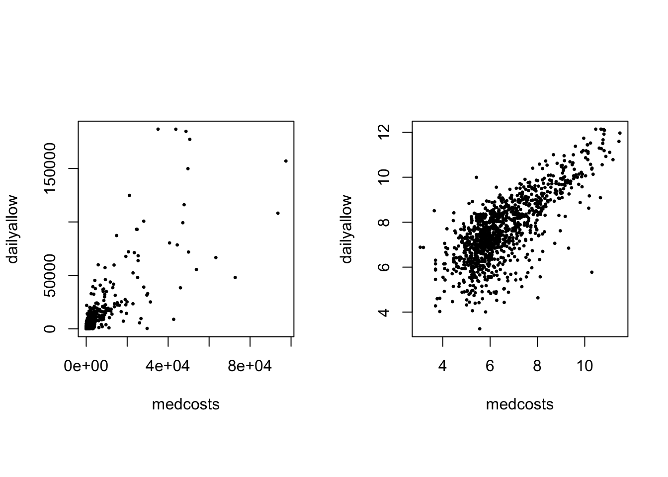
Scatterplot of those 1089 common claims (LHS) amd their log (RHS):
par(mfrow = c(1, 2), pty = "s")
plot(exp(SUVAcom), pch = 20, cex = 0.5)
plot(SUVAcom, pch = 20, cex = 0.5)
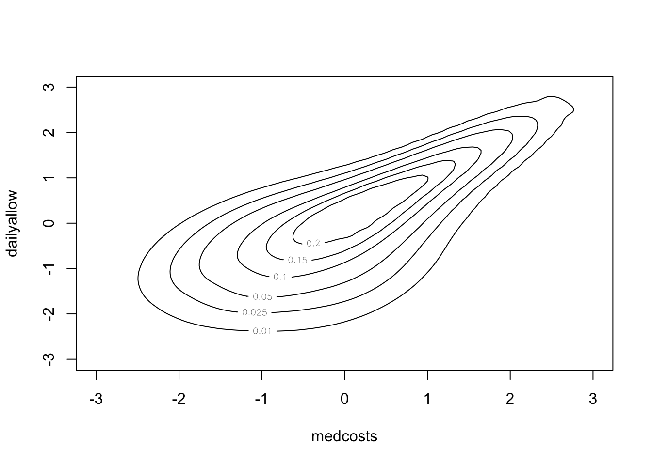
Scatterplot of the log of the 1089 common claims (LHS) and their empirical copula (ranks) (RHS):
par(mfrow = c(1, 2), pty = "s")
plot(SUVAcom, pch = 20, cex = 0.5)
plot(copula::pobs(SUVAcom)[, 1], copula::pobs(SUVAcom)[, 2],
  pch = 20, cex = 0.5)
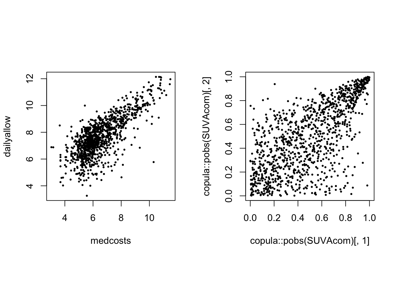
There is obvious right tail dependence.
Multivariate Normal Distributions #
The multivariate Normal distribution #
\(\mathbf{Z}=\left( Z_{1},...Z_{n}\right) ^{\prime }\sim\) \(MN\left(\mathbf{0},\Sigma \right)\) if its joint p.d.f. is \(f\left(z_{1},...,z_{n}\right) =\dfrac{1}{\sqrt{\left( 2\pi \right)^{n}\left\vert \Sigma\right\vert }}\exp \left\{-\frac{1}{2}\mathbf{z}^{\prime } \Sigma^{-1}\mathbf{z}\right\}\).
- standard Normal marginals, i.e.
\(Z_{i}\sim N\left( 0,1\right)\) - positive definite correlation matrix:
$$
\Sigma =
\begin{pmatrix} 1 & \rho_{12} & \cdots & \rho_{1n} \\ \rho_{21} & 1 & \cdots & \rho_{2n} \\ \vdots & \vdots & \ddots & \vdots \\ \rho_{n1} & \rho_{n2} & \cdots & 1 \end{pmatrix}
$$
where \(\rho_{ij} = \rho_{ji}\) is the correlation between \(Z_{i}\)
and \(Z_{j}\).
- if
\(\rho _{ij}=0\)for all\(i\neq j\), then we have the standard MN.
Properties #
If \(\mathbf{Z}\sim MN\left(\mathbf{0},{\Sigma }\right)\), then with appropriate dimensions \(\mathbf{A}\) and \(\mathbf{C}\), the vector
$$\mathbf{X=AZ+C}$$
has a multivariate Normal distribution with mean
$$\text{E}\left( \mathbf{X}\right) =\mathbf{C}$$
and covariance
$$\text{Cov}\left( \mathbf{X}\right) = \mathbf{A} \Sigma\mathbf{A}^\prime.$$
\(\adv\) Cholesky’s decomposition
#
We can construct a lower triangular matrix
$$B = \begin{pmatrix} b_{11} & 0 & \cdots & 0 \\ b_{21} & b_{22} & \cdots & 0 \\ \vdots & \vdots & \ddots & \vdots \\ b_{n1} & b_{n2} & \cdots & b_{nn} \end{pmatrix}$$
such that \(\Sigma =\mathbf{BB}^{\top}\).
The matrix \(\mathbf{B}\) can be determined using Cholesky’s decomposition algorithm (standard function in most software—see chol() in R).
This will be useful later on for the simulation of multivariate Gaussian random variables.
Measures of dependence #
Pearson’s correlation measure #
Pearson’s correlation coefficient is defined by
$$\rho \left( Z_{i},Z_{j}\right) =\rho _{ij}=\frac{\text{Cov}\left( Z_{i},Z_{j}\right) }{\sqrt{\text{Var}\left( Z_{i}\right) \text{Var}\left( Z_{j}\right) }}.$$
Note:
- This measures the degree of linear relationship between
\(Z_i\)and\(Z_j\). - In general, it does not reveal all the information on the dependence structure of random couples.
Kendall’s tau #
Kendall’s tau correlation coefficient is defined by
$$\begin{array}{rcl} \tau \left( Z_{i},Z_{j}\right) &=& \tau _{ij} \\ &=&P\left[ \left( Z_{i}-Z_{i}^{\prime }\right) \left( Z_{j}-Z_{j}^{\prime }\right) >0\right] -P\left[ \left( Z_{i}-Z_{i}^{\prime }\right) \left( Z_{j}-Z_{j}^{\prime }\right) <0\right] \end{array}$$
where \(\left( Z_{i},Z_{j}\right)\) and \(\left( Z_{i}^{\prime},Z_{j}^{\prime }\right)\) are two independent realisations.
Note:
- The first term is called the probability of concordance; the latter, probability of discordance.
- Its value is also between -1 and 1.
- It can be shown to equal:
\(\tau \left( Z_{i},Z_{j}\right) =4E\left[F\left( Z_{i},Z_{j}\right) \right] -1\). - Concordance and discordance only depends on ranks, and this indicator is hence less affected by the marginal distributions of
\(Z_i\)and\(Z_j\)
than Pearson’s correlation.
(Spearman’s) rank correlation #
Spearman’s rank correlation coefficient is defined by
$$r\left( Z_{i},Z_{j}\right) =r_{ij}=\rho \left( F_{i}\left( Z_{i}\right) ,F_{j}\left( Z_{j}\right) \right)$$
where \(F_{i}\) and \(F_{j}\) are the respective marginal distributions.
Note:
- It is indeed the Pearson’s correlation but applied to the transformed
variables
\(F_{i}\left( Z_{i}\right)\)and\(F_{j}\left( Z_{j}\right)\). - Its value is also between -1 and 1.
- It is directly formulated on ranks, and hence is less affected by the marginal distributions of
\(Z_i\)and\(Z_j\)than Pearson’s correlation.
Example: the case of multivariate Normal #
-
Pearson’s correlation:
$$\rho _{ij}$$ -
Kendall’s tau:
$$\tau _{ij}=\dfrac{2}{\pi }\arcsin \left( \rho_{ij}\right)$$ -
Spearman’s rank correlation:
$$r_{ij}=\dfrac{6}{\pi }\arcsin \left(\dfrac{\rho _{ij}}{2}\right)$$
Example: SUVA data #
cor(SUVAcom, method = "pearson") # default
##             medcosts dailyallow
## medcosts   1.0000000  0.7489701
## dailyallow 0.7489701  1.0000000
cor(SUVAcom, method = "kendall")
##             medcosts dailyallow
## medcosts   1.0000000  0.5154526
## dailyallow 0.5154526  1.0000000
cor(SUVAcom, method = "spearman")
##             medcosts dailyallow
## medcosts   1.0000000  0.6899156
## dailyallow 0.6899156  1.0000000
Repeating those on the original claims (before \(\log\) transformation):
cor(exp(SUVAcom), method = "pearson") # default
##             medcosts dailyallow
## medcosts   1.0000000  0.8015752
## dailyallow 0.8015752  1.0000000
cor(exp(SUVAcom), method = "kendall")
##             medcosts dailyallow
## medcosts   1.0000000  0.5154526
## dailyallow 0.5154526  1.0000000
cor(exp(SUVAcom), method = "spearman")
##             medcosts dailyallow
## medcosts   1.0000000  0.6899156
## dailyallow 0.6899156  1.0000000
We see that Kendall’s \(\tau\) and Spearman’s \(r\) are unchanged. This is because the \(\log\) transformation does not affect ranks in the data. The more extreme nature of the data, however, leads to a higher Pearson’s correlation coefficient.
Limits of correlation #
Correlation = dependence? #
Correlation between the consumption of cheese and deaths by becoming tangled in bedsheets (in the US, see Vigen 2015):
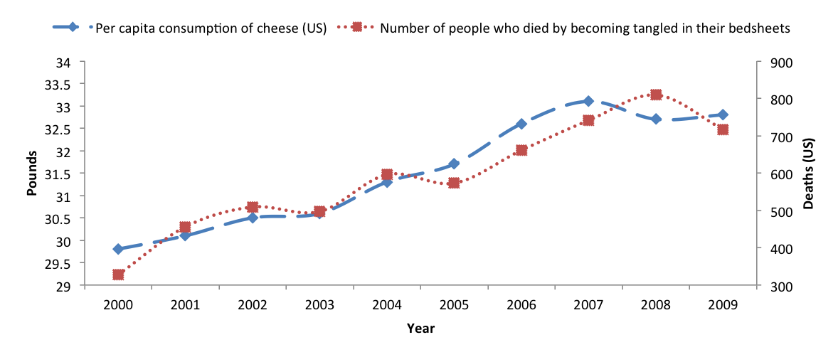
Correlation = 0.95!!
Common fallacies #
Fallacy 1: a small correlation \(\rho(X_1,X_2)\) implies that \(X_1\) and \(X_2\) are close to being independent
- wrong!
- Independence implies zero correlation BUT
- A correlation of zero does not always mean independence.
- See example 1 below.
Fallacy 2: marginal distributions and their correlation matrix uniquely determine the joint distribution.
- This is true only for elliptical families (including multivariate normal), but wrong in general!
- See example 2 below.
Example 1 #
Company’s two risks \(X_1\) and \(X_2\)
- Let
\(Z\sim N(0,1)\)and\(\Pr(U=-1)=1/2=\Pr(U=1)\) \(U\)stands for an economic stress generator, independent of\(Z\)- Consider:
$$X_1=Z\sim N(0,1)$$and$$X_2=UZ\sim N(0,1).$$Now Cov$(X_1,X_2)=E(X_1X_2)=E(UZ^2)=E(U)E(Z^2)=0$ hence\(\rho(X_1,X_2)=0\). However,\(X_1\)and\(X_2\)are strongly dependent, with 50% probability co-monotone and 50% counter-monotone.
This example can be made more realistic
Example 2 #
Marginals and correlations—not enough to completely determine joint distribution
Consider the following example:
- Marginals: Gamma
\(\left( 5,1\right)\) - Correlation:
\(\rho =0.75\) - Different dependence structures: Normal copula vs Cook-Johnson copula
- More generally, check the
Copulatheque
Example 2 illustration: Normal vs Cook-Johnson copulas #
Copula theory #
What is a copula? #
Sklar’s representation theorem #
The copula couples, links, or connects the joint distribution to its marginals.
Sklar (1959): There exists a copula function \(C\) such that
$$F\left( x_{1},x_{2},...,x_{n}\right) =C\left( F_{1}\left( x_{1}\right) ,F_{2}\left( x_{2}\right) ,...,F_{n}\left( x_{n}\right) \right)$$
where \(F_{k}\) is the marginal df of \(X_{k}\), \(k=1,2,...,n\). Equivalently,
$$\Pr\left( X_{1}\leq x_{1},...,X_{n}\leq x_{n}\right) =C\left( \Pr\left[ X_{1}\leq x_{1}\right] ,...,\Pr\left[ X_{n}\leq x_{n}\right] \right) .$$
In the case of independence,
$$F\left( x_{1},x_{2},...,x_{n}\right) = F_{1}\left( x_{1}\right) \cdot F_{2}\left( x_{2}\right) \cdots F_{n}\left( x_{n}\right)$$
so that
$$C(u_1,u_2,\ldots,u_n) = u_1 \cdot u_2 \cdots u_n.$$
Under certain conditions, the copula
$$C\left( u_{1},...,u_{n}\right) =F\left( F_{1}^{-1}\left( u_{1}\right) ,...,F_{n}^{-1}\left( u_{n}\right) \right),\quad 0\le u_1,u_2,\ldots,u_n \le 1,$$
is unique, where \(F_{k}^{-1}\) denote the quantile functions.
Note:
- This is one way of constructing copulas.
- These are called implicit copulas.
- Elliptical copulas are a prominent example (e.g., Gaussian copula)
Example #
Let
$$F(x,y) = \left\{\begin{array}{cl} \displaystyle \frac{(x+1)(e^y-1)}{x+2e^{y}-1} & (x,y) \in [-1,1]\times[0,\infty] \\\\ 1-e^{-y} & (x,y)\in(1,\infty]\times[0,\infty] \\\\ 0 & \text{elsewhere} \end{array}\right.$$
Hence
$$\begin{array}{rcl} F(x,\infty)=F(x) &=& \displaystyle \frac{x+1}{2}(\equiv u), \quad x\in[-1,1] \\\\ F^{-1}(u) &=& 2u-1 = x \\\\ F(1,y)=G(y) &=& 1-e^{-y}(\equiv v),\quad y\ge 0 \\\\ G^{-1}(v) &=& -\ln (1-v) = y \end{array}$$
Finally,
$$\begin{array}{rcl} C(u,v) &=& \displaystyle \frac{(2u-1+1)[(1-v)^{-1}-1]}{2u-1+2(1-v)^{-1}-1} =\displaystyle \frac{2u (1-1+v)}{(2u-2)(1-v)+2} \\\\ &=&\displaystyle \frac{2uv}{2u-2uv-2+2v+2} =\displaystyle \frac{uv}{u+v-uv} \\\\ &=&\displaystyle uv \times \frac{1}{u+v-uv} \end{array}$$
Note:
- Independence copula is
\(C\left( u,v\right) =uv\), here “tweaked” by a function of\(u\)and\(v\) - The copula captures the dependence structure, while separating the effects of the marginals (which are behind probabilities
\(u\)and\(v\)). - Other copulas generally contain parameter(s) to fine-tune
the (strength of) dependence.
When is \(C\) a valid copula?
#
For \(n=2\), \(C\) is a function mapping \(\left[ 0,1\right] ^{2}\) to \(\left[ 0,1\right]\) that is non-decreasing and right continuous, and:
\(\lim_{u_{k}\rightarrow 0}C\left( u_{1},u_{2}\right) =0\)for\(k=1,2\);\(\lim_{u_{1}\rightarrow 1}C\left( u_{1},u_{2}\right) =u_{2}\)and\(\lim_{u_{2}\rightarrow 1}C\left( u_{1},u_{2}\right) =u_{1}\); and\(C\)satisfies the inequality\(C\left( v_{1},v_{2}\right) -C\left(u_{1},v_{2}\right) -C\left( v_{1},u_{2}\right) +C\left(u_{1},u_{2}\right) \geq 0\)for any\(u_{1}\leq v_{1},u_{2}\leq v_{2}\).
Corresponding heuristics are:
- If the event on one variable is impossible, then the joint probability is impossible.
- If the event on one variable is certain, then the joint probability boils down to the marginal of the other one.
- There cannot be negative probabilities.
\(\adv\) Multivariate distribution function
#
We will now generalise this to \(n\ge 2\) by first recalling the properties of a multivariate df.
A function \(F:R^{n}\rightarrow \lbrack 0,1]\) is a multivariate d.f. if
it satisfies:
- right-continuous;
\(\lim_{x_{i}\rightarrow -\infty }F\left( x_{1},...,x_{n}\right) =0\)for\(i=1,2,...,n;\)\(\lim_{x_{i}\rightarrow \infty ,\forall i}F\left(x_{1},...,x_{n}\right) =1;\)and- rectangle inequality holds: for all
\(\left( a_{1},...,a_{n}\right)\)and\(\left( b_{1},...,b_{n}\right)\)with\(a_{i}\leq b_{i}\)for\(i=1,...,n\), we have
$$\sum_{i_{1}=1}^{2}\cdots \sum_{i_{n}=1}^{2}\left( -1\right) ^{i_{1}+\cdots +i_{n}}F\left( x_{1i_{1}},...,x_{ni_{n}}\right) \geq 0,$$
where \(x_{i1}=a_{i}\) and \(x_{i2}=b_{i}\).
\(\adv\) Multivariate copula
#
A copula \(C:[0,1]^{n}\rightarrow \lbrack 0,1]\) is a multivariate
distribution function whose univariate marginals are Uniform \((0,1)\) .
Properties of a multivariate copula:
\(C\left( u_{1},...,u_{k-1},0,u_{k+1},...,u_{n}\right) =0\)\(C\left( 1,...,1,u_{k},1,...,1\right) =u_{k}\)- the rectangle inequality leads us to
$$\begin{array}{rcl} &&P\left( a_{1}\leq U_{1}\leq b_{1},...,a_{n}\leq U_{n}\leq b_{n}\right) \\ &=&\displaystyle \sum_{i_{1}=1}^{2}\cdots \sum_{i_{n}=1}^{2}\left( -1\right) ^{i_{1}+\cdots +i_{n}}C\left( u_{1i_{1}},...,u_{ni_{n}}\right) \geq 0 \end{array}$$
for all \(u_{i}\in \lbrack 0,1]\), \(\left( a_{1},...,a_{n}\right)\) and \(\left( b_{1},...,b_{n}\right)\) with \(a_{i}\leq b_{i},\) and
\(u_{i1}=a_{i}\) and \(u_{i2}=b_{i}.\)
Heuristics are the same as before.
Density associated with a copula #
For continuous marginals with respective pdf \(f_{1},...f_{n}\), the
joint pdf of \(\mathbf{X}\) can be written as
$$f\left( x_{1},...,x_{n}\right) =f_{1}\left( x_{1}\right) \cdot \cdot \cdot f_{n}\left( x_{n}\right) \times c\left( F_{1}\left( x_{1}\right) ,...,F_{n}\left( x_{n}\right) \right)$$
where the copula density \(c\) is given by
$$c\left( u_{1},...,u_{n}\right) =\frac{\partial ^{n}C\left( u_{1},...,u_{n}\right) }{\partial u_{1}\partial u_{2}\cdot \cdot \cdot \partial u_{n}}.$$
Note:
- The copula
\(c\)distorts the independence case to induce the actual dependence structure. - If independent,
\(c\left( u_{1},...,u_{n}\right)=1\).
Example #
Let \(X\) and \(Y\) be two random variables and the copula \(C\) of \(X\) and \(Y\) is
$$C(u,v)=\frac{uv}{u+v-uv}.$$
Derive its associated density \(c\).
Survival copulas #
What if we want to work with (model) survival functions
$$\overline{F}_i(x_i)=1-F_i(x_i)\left(=S_i(x_i)\right)$$
rather than distribution functions?
\(\longrightarrow\) We can couple \(\overline{F}_i\)’s with the survival copulas \(\overline{C}\).
In the bivariate case, this yields
$$\overline{F}(x_1,x_2)=\Pr[X_1>x_1,X_2>x_2]=\overline{C}\left(\overline{F}_1(x_1),\overline{F}_2(x_2)\right),$$
where
$$\overline{C}(1-u,1-v)=1-u-v+C(u,v).$$
This is because
$$\begin{array}{rcl} \Pr[X_1>x_1,X_2>x_2]&=&1-\Pr[X_1 \le x_1]-\Pr[X_2 \le x_2] \\ &&+\Pr[X_1\le x_1,X_2\le x_2]. \end{array}$$
Invariance property #
- Suppose random vector
\(\mathbf{X}\)has copula\(C\)and suppose\(T_{1},...,T_{n}\)are non-decreasing continuous functions of\(X_{1},...,X_{n}\), respectively. - The random vector defined by
\(\left( T_{1}\left( X_{1}\right),...,T_{n}\left( X_{n}\right) \right)\)has the same copula\(C\).
Proof: see Theorem 2.4.3 (p. 25) of Nelsen (1999) - The usefulness of this property can be illustrated in many ways. If you have a copula describing joint distribution of insurance losses of various types, and you decide the quantity of interest is a transformation (e.g. logarithm) of these losses, then the multivariate distribution structure does not change.
- The copula is then also invariant to inflation.
- Only the marginal distributions change.
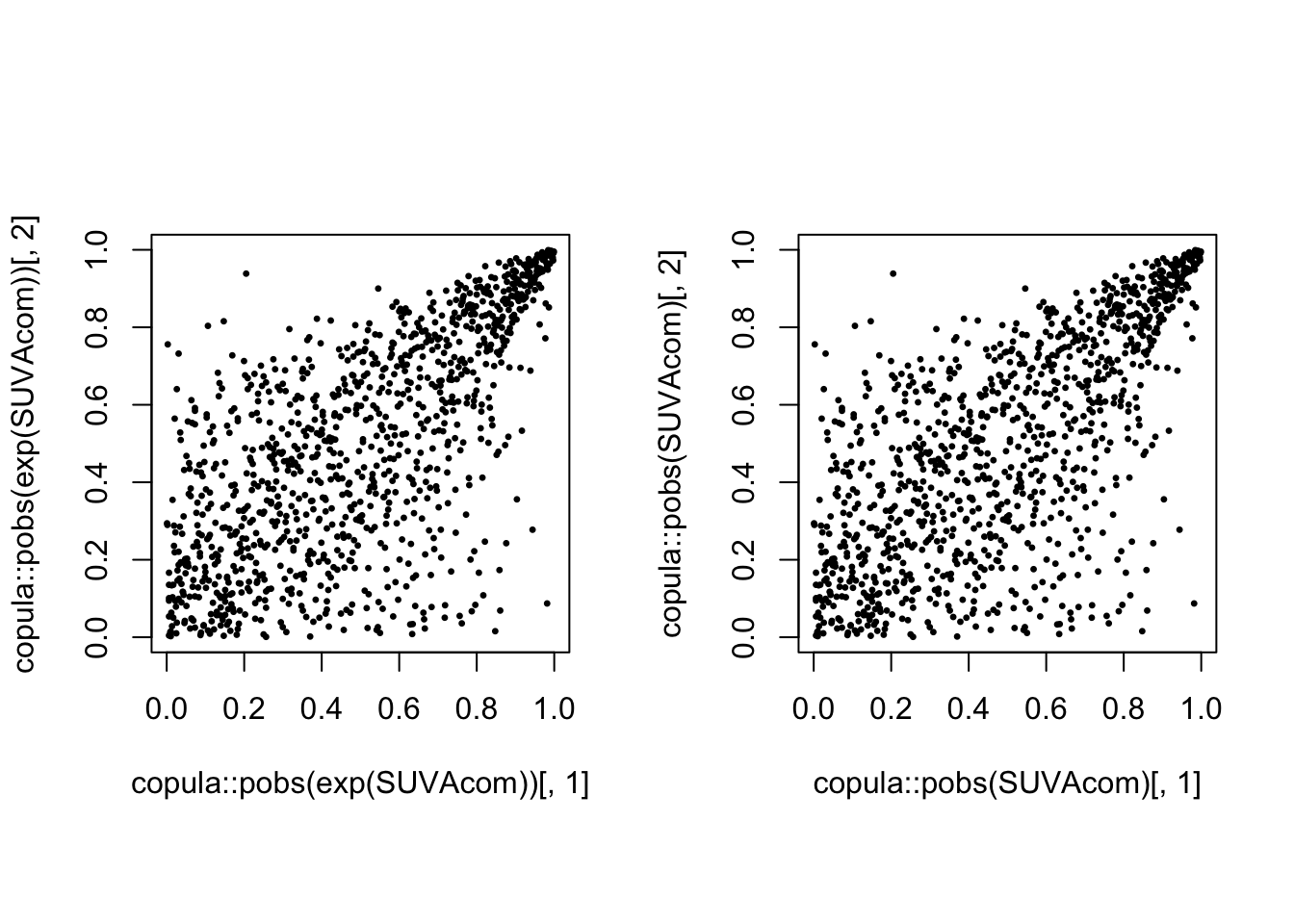
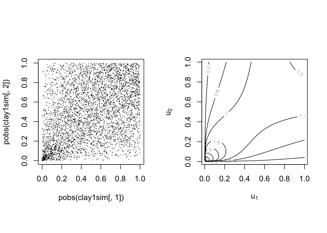
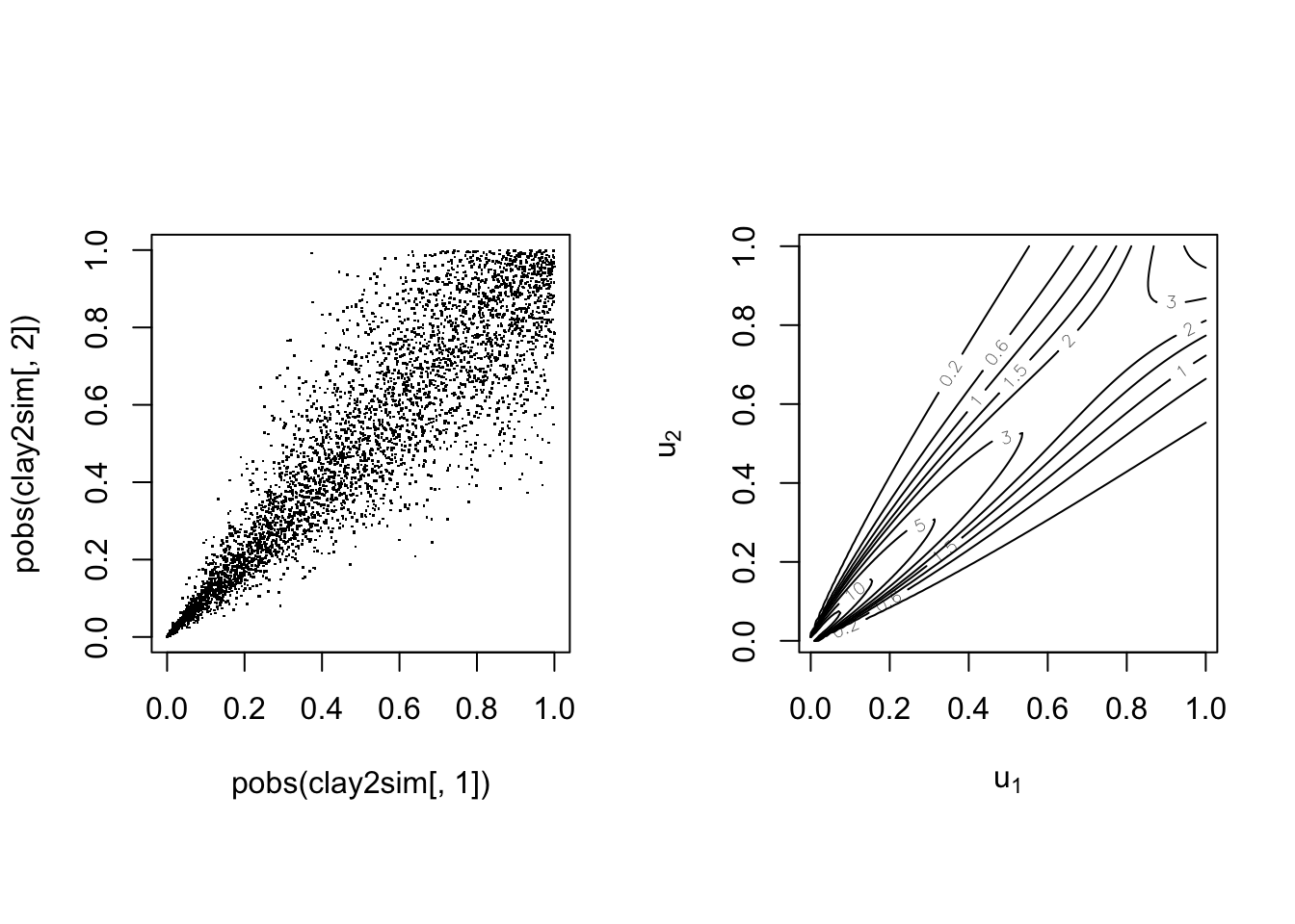
Empirical copula of the 1089 common claims (LHS) and of their log (RHS):
par(mfrow = c(1, 2), pty = "s")
plot(copula::pobs(exp(SUVAcom))[, 1], copula::pobs(exp(SUVAcom))[,
  2], pch = 20, cex = 0.5)
plot(copula::pobs(SUVAcom)[, 1], copula::pobs(SUVAcom)[, 2],
  pch = 20, cex = 0.5)
Main bivariate copulas #
The Fréchet bounds #
Define the Fréchet bounds as:
- Fréchet lower bound:
\(L_{F}\left( u_{1},...,u_{n}\right) =\max \left(\sum_{k=1}^{n}u_{k}-\left( n-1\right) ,0\right)\) - Fréchet upper bound:
\(U_{F}\left( u_{1},...,u_{n}\right) =\min \left(u_{1},...,u_{n}\right)\)
Any copula function satisfies the following bounds:
$$L_{F}\left( u_{1},...,u_{n}\right) \leq C\left(u_{1},...,u_{n}\right) \leq U_{F}\left( u_{1},...,u_{n}\right).$$
The Fréchet upper bound satisfies the definition of a copula, but the
Fréchet lower bound does not for dimensions \(n\geq 3\).
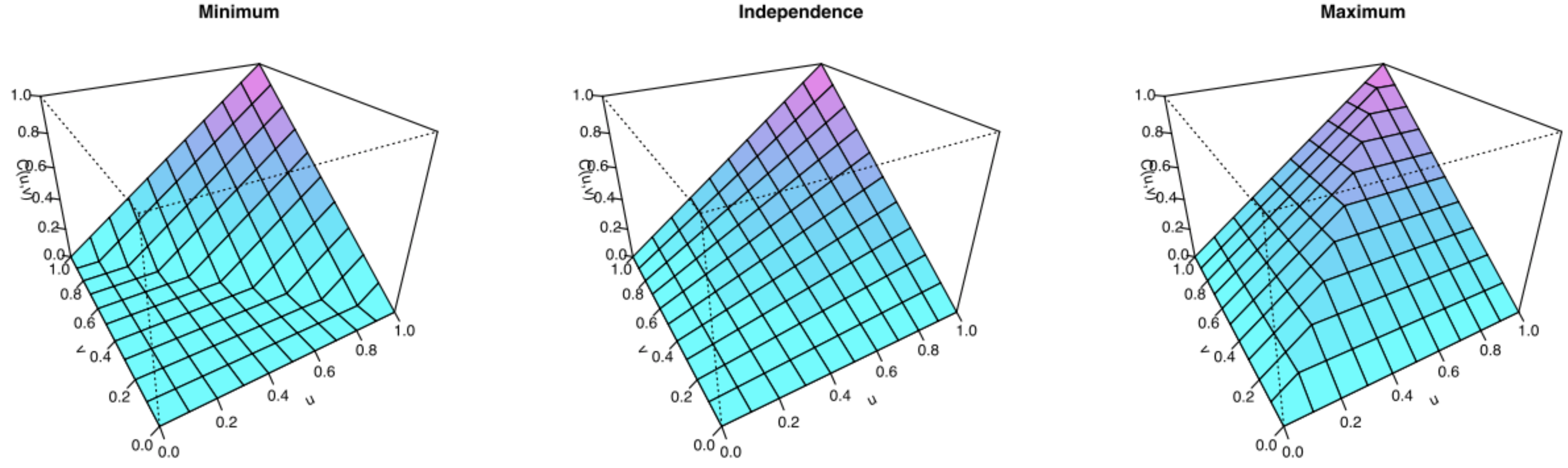
Source: Wikipedia (2020)
The Normal (aka Gaussian) copula #
Recall that \(\mathbf{Z}=\left( Z_{1},...Z_{n}\right) ^{\prime }\sim\)
\(MN\left( \mathbf{0},\Sigma \right)\) if its joint p.d.f.
is
$$f\left(z_{1},...,z_{n}\right)=\frac{1}{\sqrt{\left( 2\pi \right) ^{n} \vert \Sigma \vert }}\exp \left[ -\frac{1}{2} \mathbf{z}^{\prime }\Sigma^{-1}\mathbf{z}\right]$$
where \(\mathbf{z}=\left( z_{1},...z_{n}\right)\).
Now define its joint distribution by
$$\Phi_{\Sigma}\left( z_{1},...,z_{n}\right) = \int_{-\infty }^{z_{n}}\int_{-\infty }^{z_{n-1}}\cdot \cdot \cdot \int_{-\infty }^{z_{1}} \frac{1}{\sqrt{\left( 2\pi \right)^{n} \vert \Sigma \vert }}\exp \left[ -\frac{1}{2}\mathbf{z}^{\prime }\Sigma^{-1}\mathbf{z}\right] dz_{1}\cdot \cdot \cdot dz_{n}$$
Let \(\Phi(\cdot)\) denote the standard normal cumulative distribution function. The copula defined by
$$C\left( u_{1},...,u_{n}\right) =\Phi _{\Sigma}\left( \Phi ^{-1}\left( u_{1}\right) ,...,\Phi ^{-1}\left( u_{n}\right) \right)$$
is called the Normal (or Gaussian) copula.
Illustration of the Gaussian copula:
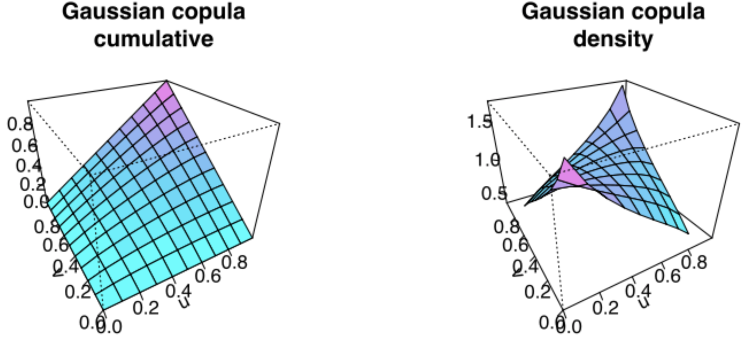
Here \(\rho=0.4\). Source: Wikipedia (2020)
The \(t\) copula
#
A r vector \(\mathbf{Z}=\left( Z_{1},...Z_{n}\right) ^{\prime}\sim MT \left( \mathbf{0},\Sigma;\upsilon \right)\) if its joint p.d.f. is
$$f\left( z_{1},...,z_{n}\right) = \frac{\Gamma \left( \frac{\upsilon +1}{2} \right) }{\sqrt{\left( \upsilon \pi \right) ^{n}\left\vert \Sigma \right\vert }\Gamma \left( \frac{\upsilon }{2}\right) }\left( 1+\frac{1}{ \upsilon }\mathbf{z}^{\prime }\Sigma^{-1}\mathbf{z}\right) ^{-(\upsilon +n)/2}.$$
Now define its joint distribution by
$$T_{\Sigma ,\upsilon }\left( z_{1},...,z_{n}\right) =\int_{-\infty }^{z_{n}}\int_{-\infty }^{z_{n-1}}\cdot \cdot \cdot \int_{-\infty }^{z_{1}} \frac{\Gamma \left( \frac{\upsilon +1}{2}\right) }{\sqrt{\left( \upsilon \pi \right) ^{n}\left\vert \Sigma\right\vert }\Gamma \left( \frac{ \upsilon }{2}\right) }\left( 1+\frac{1}{\upsilon }\mathbf{z}^{\prime } \Sigma^{-1}\mathbf{z}\right) ^{-(\upsilon +n)/2}dz_{1}\cdot \cdot \cdot dz_{n}.$$
Let \(t_{\upsilon }(\cdot)\) denote the cumulative distribution function of a standard univariate \(t\) distribution. The copula defined by
$$C\left( u_{1},...,u_{n}\right) =T_{\Sigma ,\upsilon }\left( t_{\upsilon }^{-1}\left( u_{1}\right) ,...,t_{\upsilon }^{-1}\left( u_{n}\right) \right)$$
is called the \(t\) copula.
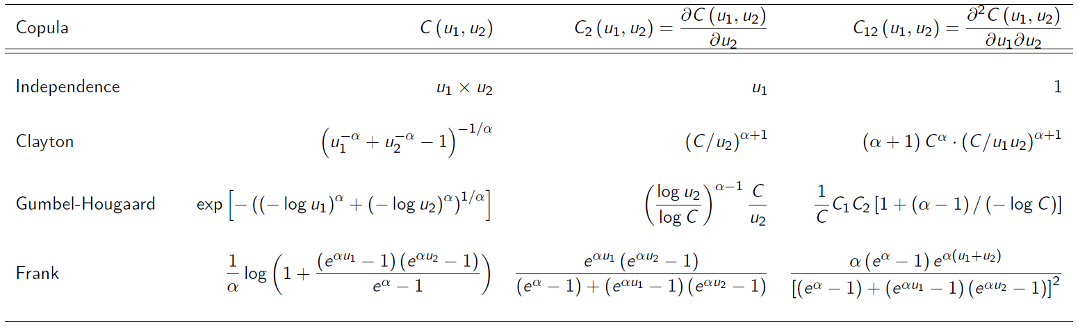
Archimedean copulas #
\(C\) is Archimedean if it has the form
$$C\left( u_{1},...,u_{n}\right) =\psi ^{-1}\left( \psi \left( u_{1}\right) +\cdots+\psi \left( u_{n}\right) \right)$$
for all \(0\leq u_{1},...,u_{n}\leq 1\) and for some function \(\psi\)
(called the generator) satisfying:
\(\psi \left( 1\right) =0;\)\(\psi\)is decreasing; and\(\psi\)is convex.
The Clayton copula #
The Clayton copula is defined by
$$C\left( u_{1},...,u_{n}\right) =\left( \sum_{k=1}^{n}u_{k}^{-\theta }-n+1\right) ^{-1/\theta }, \quad \theta \in (0,\infty)$$
It is of Archimedean type with:
\(\psi \left( t\right) =\frac{1}{\theta}(t^{-\theta }-1)\)\(\psi ^{-1}\left( s\right) =\left( 1+\theta s\right) ^{-1/\theta }\)
Note the correspondance with Kendall’s \(\tau\) (for bivariate case):
$$\theta = \frac{2\tau}{1-\tau} \quad \Longleftrightarrow \quad \tau = \frac{\theta}{2+\theta}$$
This copula is asymmetric with positive dependence in the left tail.
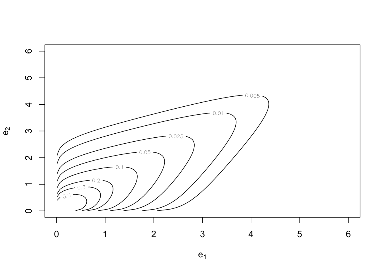
The Clayton copula for \(n=2\)
#
We have
$$C\left( u_{1},u_{2}\right) =\left( u_{1}^{-\theta }+u_{2}^{-\theta}-1\right) ^{-1/\theta }$$
With parameter \(\tau=0.25\)
With parameter \(\tau=0.75\)
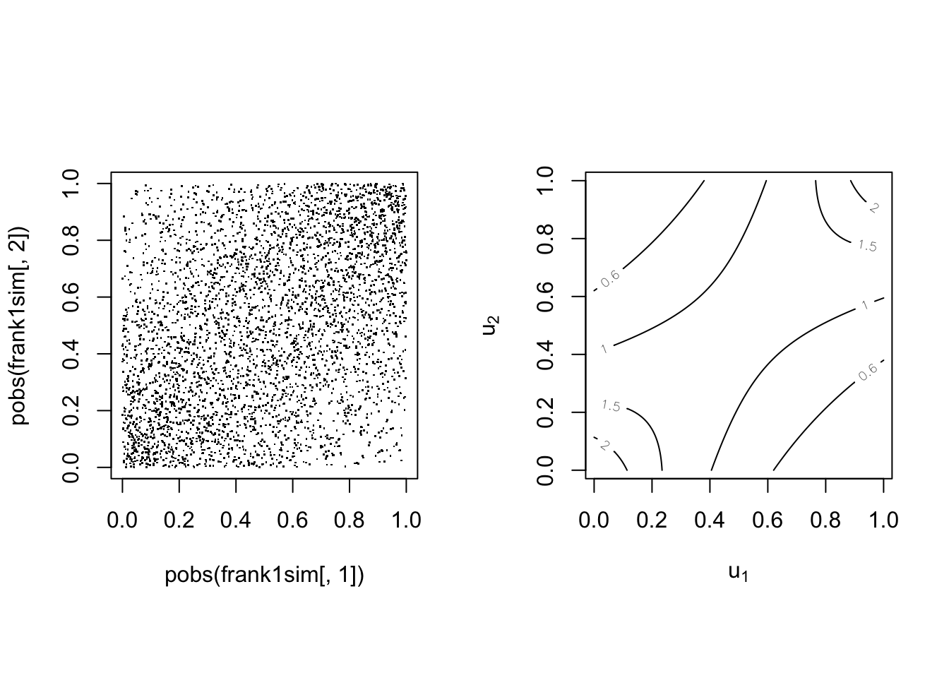
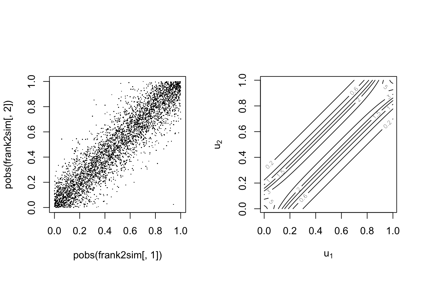
The Frank copula #
The Frank copula is defined by
$$C\left( u_{1},...,u_{n}\right) = \dfrac{1}{\theta }\log \left( 1+\dfrac{\prod_{i=1}^n\left( e^{\theta u_{i}}-1\right) }{e^{\theta}-1}\right) , \quad \theta \in \mathbb{R} \backslash \{0\} %C\left( u_{1},...,u_{n}\right) = \dfrac{1}{\alpha }\log \left( 1+\dfrac{\left( e^{\alpha u_{1}}-1\right) \left( e^{\alpha u_{2}}-1\right) }{e^{\alpha}-1}\right) %\frac{1}{\log \theta }\log \left(1+\frac{ \prod\nolimits_{k=1}^{n}\left( \theta ^{u_{k}}-1\right)}{\left( \theta -1\right) ^{n-1}}\right) , \quad \theta \in \mathbb{R}^+ \backslash \{1\}$$
It is of Archimedean type with:
\(\psi \left( t\right) =-\log \left( \frac{e ^{-\theta t}-1}{e^{-\theta} -1}\right)\)\(\psi ^{-1}\left( s\right) =-\frac{1}{\theta }\log \left(1+e^{-s}\left( e^{-\theta}-1\right) \right)\)
Note the correspondance with Kendall’s \(\tau\) (for bivariate case):
$$\tau = 1-\frac{4}{\theta}+\frac{4}{\theta^2}\int_0^\theta \frac{t}{e^t-1}dt.$$
This copula is symmetric.
With parameter \(\tau=0.25\)
With parameter \(\tau=0.75\)
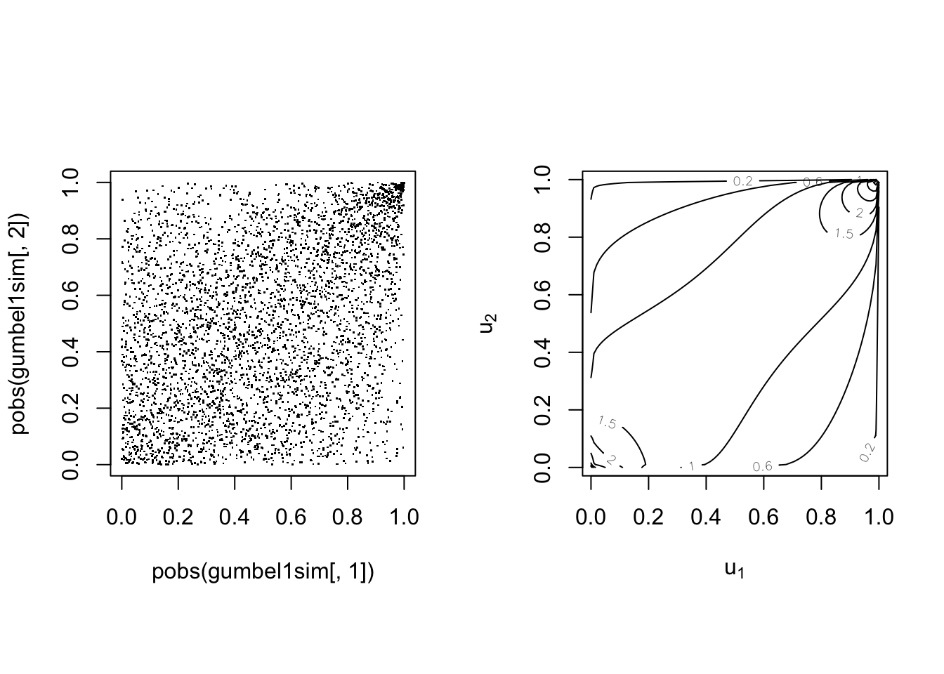
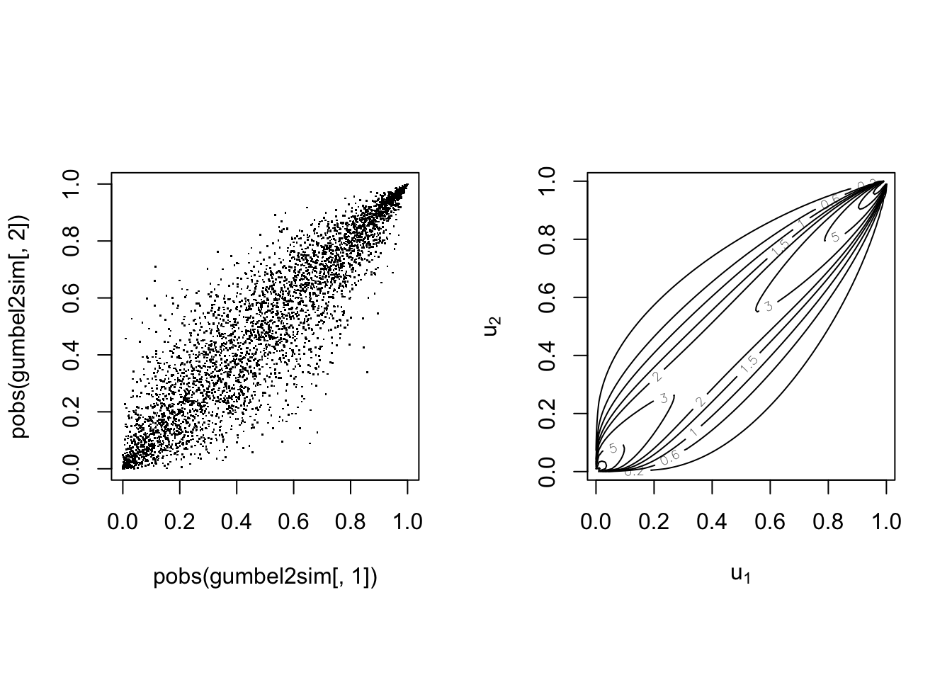
The Gumbel(-Hougard) copula #
The Gumbel copula is defined by
$$C\left( u_{1},...,u_{n}\right) = \exp \left[ -\left(\sum_{i=1}^n (-\log u_i)^\theta\right)^{1/\theta}\right] \,\quad \theta \in [1,\infty)$$
It is of Archimedean type with:
\(\psi \left( t\right) = \left( -\log t \right)^\theta\)\(\psi ^{-1}\left( s\right) =\exp\left\{ -t^{1/\theta}\right\}\)
Note correspondance with Kendall’s \(\tau\) (for bivariate case):
$$\theta = \frac{1}{1-\tau} \quad \Longleftrightarrow \quad \tau = \frac{\theta-1}{\theta}$$
This copula is asymmetric with greater dependence in the right tail,
which makes it often a good candidate for large claims with a
common underlying cause.
With parameter \(\tau=0.25\)
With parameter \(\tau=0.75\)
Copula models in R #
The VineCopula package
#
- The
VineCopulapackage caters for many of the basic copula modelling requirements. - Vine copulas (Kurowicka and Joe 2011) allow for the construction of multivariate copulas with flexible dependence structures; they are outside the scope of this Module.
- The package, however, has a series of modelling functions specifically designed for bivariate copula modelling via the “BiCop-family”.
BiCop: Creates a bivariate copula by specifying the family and parameters (or Kendall’s tau). Returns an object of classBiCop.The class has the following methods:print,summary: a brief or comprehensive overview of the bivariate copula, respectively.plot,contour: surface/perspective and contour plots of the copula density. Possibly coupled with standard normal margins (default for contour).
- For most functions, you can provide an object of class
BiCopinstead of specifyingfamily,parandpar2manually.
Bivariate copulas in VineCopula
#
The following bivariate copulas are available in the
VineCopula package within the bicop family:
| Copula family | family |
par |
par2 |
|---|---|---|---|
| Gaussian | 1 | (-1, 1) | - |
| Student t | 2 | (-1, 1) | (2,Inf) |
| (Survival) Clayton | 3, 13 | (0, Inf) | - |
| Rotated Clayton (90° and 270°) | 23, 33 | (-Inf, 0) | - |
| (Survival) Gumbel | 4, 14 | [1, Inf) | - |
| Rotated Gumbel (90° and 270°) | 24, 34 | (-Inf, -1] | - |
| Frank | 5 | R {0} | - |
| (Survival) Joe | 6, 16 | (1, Inf) | - |
| Rotated Joe (90° and 270°) | 26, 36 | (-Inf, -1) | - |
| Copula family | family |
par |
par2 |
|---|---|---|---|
| (Survival) Clayton-Gumbel (BB1) | 7, 17 | (0, Inf) | [1, Inf) |
| Rotated Clayton-Gumbel (90° and 270°) | 27, 37 | (-Inf, 0) | (-Inf, -1] |
| (Survival) Joe-Gumbel (BB6) | 8, 18 | [1 ,Inf) | [1, Inf) |
| Rotated Joe-Gumbel (90° and 270°) | 28, 38 | (-Inf, -1] | (-Inf, -1] |
| (Survival) Joe-Clayton (BB7) | 9, 19 | [1, Inf) | (0, Inf) |
| Rotated Joe-Clayton (90° and 270°) | 29, 39 | (-Inf, -1] | (-Inf, 0) |
| (Survival) Joe-Frank (BB8) | 10, 20 | [1, Inf) | (0, 1] |
| Rotated Joe-Frank (90° and 270°) | 30, 40 | (-Inf, -1] | [-1, 0) |
| (Survival) Tawn type 1 | 104, 114 | [1, Inf) | [0, 1] |
| Rotated Tawn type 1 (90° and 270°) | 124, 134 | (-Inf, -1] | [0, 1] |
| (Survival) Tawn type 2 | 204, 214 | [1, Inf) | [0, 1] |
| Rotated Tawn type 2 (90° and 270°) | 224, 234 | (-Inf, -1] | [0, 1] |
All of these copulas are illustrated in the
copulatheque.
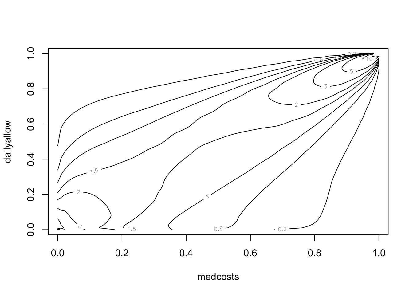
Example of Gumbel copula:
cop <- VineCopula::BiCop(4, 2)
print(cop)
## Bivariate copula: Gumbel (par = 2, tau = 0.5)
summary(cop)
## Family
## ------
## No:    4
## Name:  Gumbel
##
## Parameter(s)
## ------------
## par:  2
##
## Dependence measures
## -------------------
## Kendall's tau:    0.5
## Upper TD:         0.59
## Lower TD:         0
plot(cop)
Note this is for uniform margins.
Now with a standard normal margin:
plot(cop, type = "surface", margins = "norm")
Contour plots are done with normal margins as standard:
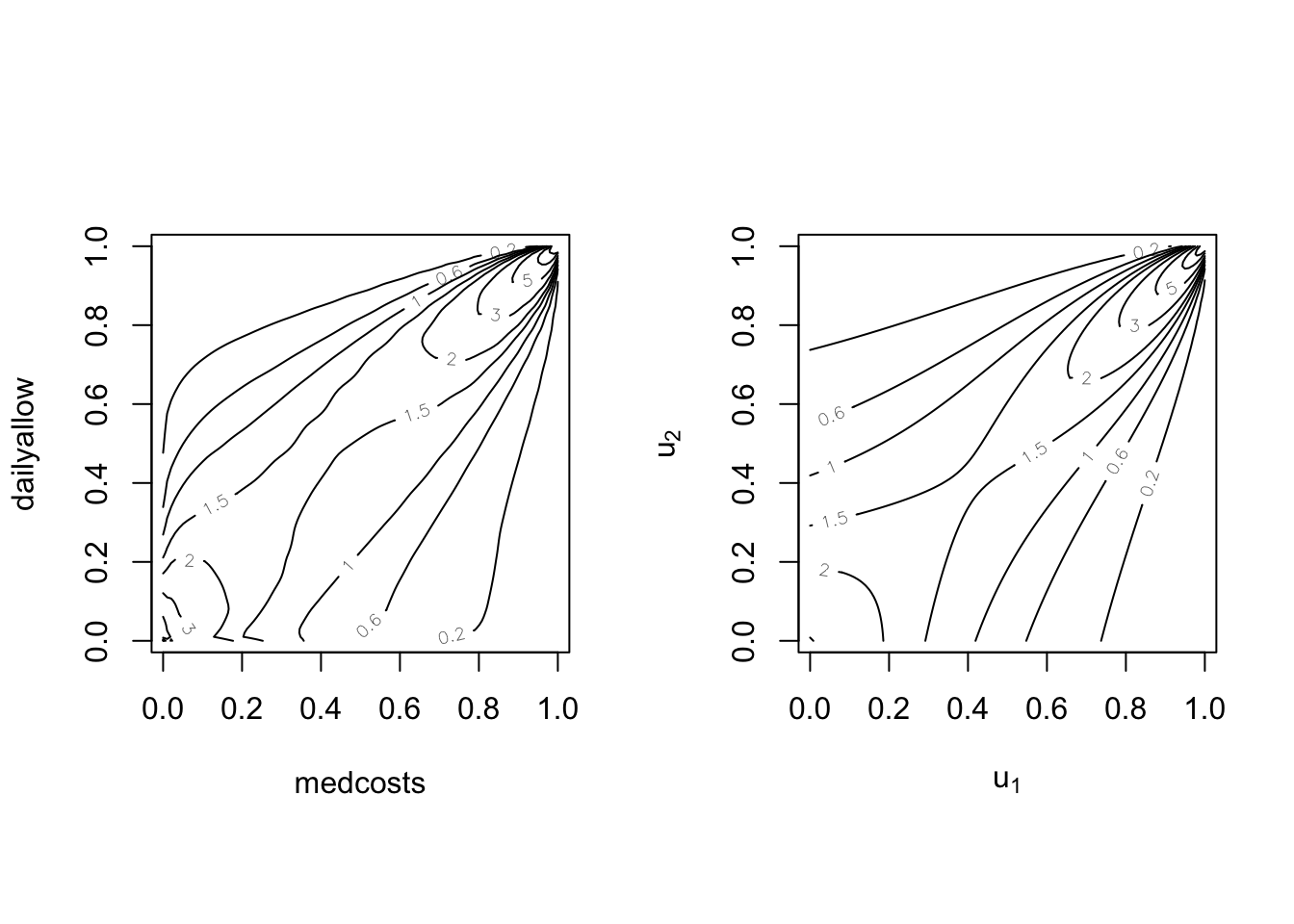
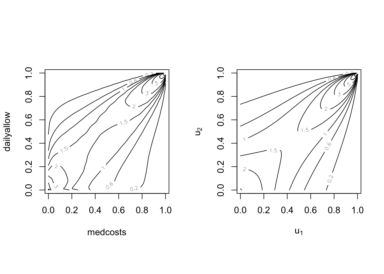
plot(cop, type = "contour")
But uniform margins are still possible:
plot(cop, type = "contour", margins = "unif")
And so are exponential margins in both cases:
plot(cop, type = "contour", margins = "exp")
Conversion between dependence measures and parameters (for a given family): #
BiCopPar2Tau: computes the theoretical Kendall’s tau value of a bivariate copula for given parameter values.BiCopTau2Par: computes the parameter of a (one parameter) bivariate copula for a given value of Kendall’s tau.
Example of conversion for Clayton:
tau <- BiCopPar2Tau(3, 2.5)
tau
## [1] 0.5555556
theta <- 2 * tau/(1 - tau)
theta
## [1] 2.5
BiCopTau2Par(3, tau)
## [1] 2.5
Evaluate functions related to a bivariate copula: #
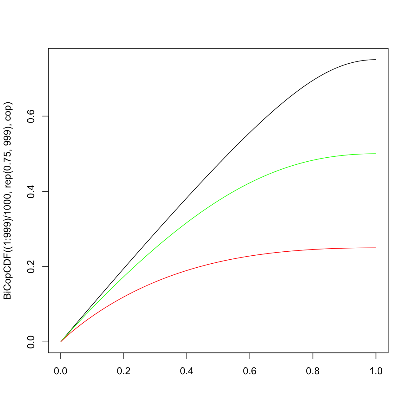
BiCopPDF/BiCopCDF: evaluates the pdf/cdf of a given parametric bivariate copula.BiCopDeriv: evaluates the derivative of a given parametric bivariate copula density with respect to its parameter(s) or one of its arguments.
plot((1:999)/1000, BiCopCDF((1:999)/1000, rep(0.75, 999), cop),
  type = "l", xlab = "")  #u_2 = 0.75
lines((1:999)/1000, BiCopCDF((1:999)/1000, rep(0.5, 999), cop),
  type = "l", col = "green")  #u_2 = 0.5
lines((1:999)/1000, BiCopCDF((1:999)/1000, rep(0.25, 999), cop),
  type = "l", col = "red")  #u_2 = 0.25
\(\adv\) Simulation from bivariate copulas
#
\(\adv\) Reminder: simulation of a univariate random variable
#
- Remember that if
\(X \in \mathbb{R}\)has distribution function\(F\)then $$ F(X) \sim \text{uniform}(0,1).$$ - This forms the basis of most simulation techniques, as a pseudo-uniform
\(u \in (0,1)\)can then be mapped into a pseudo-random\(x \in \mathbb{R}\)with df F by applying $$ x = F^{-1}(u).$$
\(\adv\) Overarching strategy
#
- We will introduce the general conditional distribution method.
- The overarching idea is (for the bivariate case):
- simulate two independent uniform random variable
\(u\)and\(t\); - “tweak”
\(t\)into a\(v\in[0,1]\)so that it has the right dependence structure (w.r.t.\(u\)) with the help of the copula; - map
\(u\)and\(v\)into marginal\(x\)and\(y\)using their distribution function.
- simulate two independent uniform random variable
- However, there are some specific, more efficient algorithms that are available for certain types of copulas (see, e.g. Nelsen 1999).
- In R, the function
BiCopSimwill simulate from a given parametric bivariate copula.
\(\adv\) Preliminary: the conditional distribution function
#
For the “tweak”, we will need the conditional distribution function for \(V\) given \(U=u\), which is denoted by \(c_u(v):\)
\begin{align*} c_u(v)&=\Pr[V\leq v|U=u] \\ &= \lim_{\Delta u \to 0}\frac{C(u+\Delta u,v)-C(u,v)}{\Delta u} \\ &=\frac{\partial C(u,v)}{\partial u}. \end{align*}
In particular, we will need its inverse.
\(\adv\) Example
#
For the copula
$$C(u,v)=\frac{uv}{u+v-uv}$$
we have
$$\begin{array}{rcl} c_u(v) &=& \displaystyle \frac{v(u+v-uv)-uv(1-v)}{(u+v-uv)^2}=\left(\frac{v}{u+v-uv}\right)^2 \equiv t \\\\ c_u^{-1}(t) &=& \displaystyle \frac{\sqrt{t}u}{1-\sqrt{t}(1-u)} \equiv v \end{array}$$
\(\adv\) In R
#
For copulas of the BiCop family:
BiCopHfunc: evaluates the conditional distribution function\(c_u(v)\)(aka h-function) of a given parametric bivariate copula.BiCopHinv: evaluates the inverse conditional distribution function\(c_u^{-1}(v)\)(aka inverse h-function) of a given parametric bivariate copula.BiCopHfuncDeriv: evaluates the derivative of a given conditional parametric bivariate copula (h-function) with respect to its parameter(s) or one of its arguments.
\(\adv\) The conditional distribution method
#
Goal: generate a pair of pseudo-random variables \((X,Y)\) with d.f.’s \(F\) and \(G\), respectively, with dependence structure described by the copula \(C\).
Algorithm
- Generate two independent uniform
\((0,1)\)pseudo-random variables\(u\)and\(t\); - Set
\(v=c_u^{-1}(t)\); - Map
\((u,v)\)into\((x,y)\):
$$\begin{array}{rcl} x &=& F^{-1}(u); \\ y &=& G^{-1}(v). \end{array}$$
\(\adv\) Example
#
Let \(X\) and \(Y\) be exponential with mean 1 and standard Normal, respectively. Furthermore, the copula describing their dependence is such as in the previous example:
$$C(u,v)=\frac{uv}{u+v-uv}$$
Furthermore, you are given the following pseudo-random (independent) uniforms:
$$0.3726791, 0.6189313, 0.75949099, 0.01801882$$
Simulate two pairs of outcomes for \((X,Y)\).
Use of the conditional distribution method yields
- We can use the uniforms given in the question such that
$$\begin{array}{rcl} (u_1,t_1) &=& (0.3726791, 0.6189313) \\ (u_2,t_2) &=& (0.75949099, 0.01801882) \end{array}$$
- Set
\(v_i=\frac{u_i\sqrt{t_i}}{1-(1-u_i)\sqrt{t_i}}\)for\(i=1,2\):
$$\begin{array}{rcl} v_1&=&0.5788953 \\ v_2&=&0.1053509 \end{array}$$
- Mapping
\((u_i,v_i)\)into\((x_i,y_i)\)using$$x_i=F^{-1}(u_i)=-\ln (1-u_i) \text{ and } y_i=\Phi^{-1}(v_i)\text{ we have}$$$$\begin{array}{rcl} (x_1,y_1) &=& (0.466297, 0.199068) \\ (x_2,y_2) &=& (1.424998, -1.251638) \end{array}$$
\(\adv\) Specific algorithms
#
The following algorithms are provided for illustration purposes. They are not assessable.
\(\adv\) Simulation from a Normal copula
#
Let \(C\) be a Normal copula. The following algorithm generates \(\left( x_{1},...,x_{n}\right)\)
from a random vector \((X_1,\cdots, X_n)\) with marginal distribution functions \(F_{X_1}(\cdot),\cdots, F_{X_n}(\cdot)\), and copula \(C\), i.e. \(Pr(X_1\le x_1,\cdots,X_n\le x_n)=C(F_{X_1}(x_1),\cdots,F_{X_n}(x_n))\):
The following algorithm generates \(\left( x_{1},...,x_{n}\right)\) from the Normal copula:
- construct the lower triangular matrix
\(\mathbf{B}\)so that the correlation matrix\(\Sigma\mathbf{=BB}^{\top}\)using Cholesky’s. - generate a column vector of independent standard Normal rv’s
\(\mathbf{Z}=\left(z_{1},...,z_{n}\right)\). - take the matrix product of
\(\mathbf{B}\)and\(\mathbf{Z}\), i.e.\(\mathbf{Y=BZ}\). - set
\(u_{k}=\Phi \left( u_{k}\right)\)for\(k=1,2,...,n.\) - set
\(x_{k}=F_{X_{k}}^{-1}\left( u_{k}\right)\)for\(k=1,2,...,n.\) \(\left( x_{1},...,x_{n}\right)\)is the desired vector with marginals\(F_{X_{k}}\)for\(k=1,...,n\)and Normal copula\(C\).
\(\adv\) Simulation from a Clayton copula
#
Let \(C\) be the Clayton copula. The following algorithm generates \(\left( x_{1},...,x_{n}\right)\)
from a random vector \((X_1,\cdots, X_n)\) with marginal distribution functions \(F_{X_1}(\cdot),\cdots, F_{X_n}(\cdot)\), and copula \(C\):
- generate a column vector of independent
\(Exp\left( 1\right)\)rv’s\(\mathbf{Y}=\left( y_{1},...,y_{n}\right)\). - generate
\(z\)from a Gamma$\left( 1/\theta ,1\right)$ distribution. - set
\(u_{k}=\left( 1+y_{k}/z\right) ^{-1/\theta }\)for\(k=1,2,...,n.\) - set
\(x_{k}=F_{X_{k}}^{-1}\left( u_{k}\right)\)for\(k=1,2,...,n.\) \(\left( x_{1},...,x_{n}\right)\)is the desired vector with marginals\(F_{X_{k}}\)for\(k=1,...,n\)and Clayton copula\(C\).
\(\adv\) Example of simulation in R
#
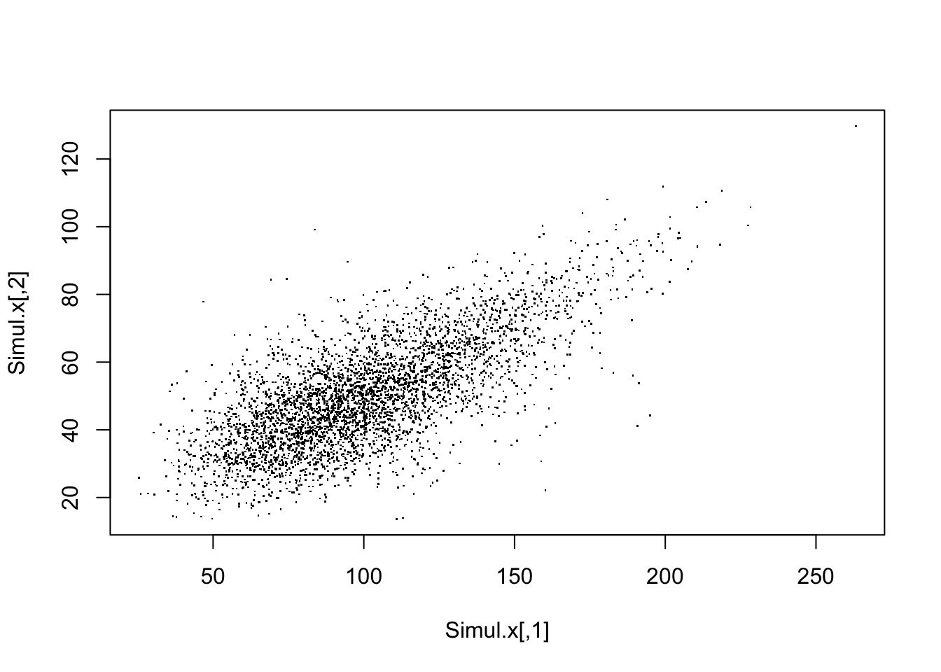
We simulate 4000 pairs \((u_1,u_2)\) from the Gumbel copula (with parameter 2) defined above:
Simul.u <- BiCopSim(4000, cop)
head(Simul.u, 15)
##             [,1]      [,2]
##  [1,] 0.50867346 0.3359880
##  [2,] 0.39195033 0.2236886
##  [3,] 0.41313775 0.4327339
##  [4,] 0.49581195 0.2732273
##  [5,] 0.06705059 0.1024408
##  [6,] 0.69906709 0.7715066
##  [7,] 0.20296035 0.2651919
##  [8,] 0.97195829 0.9397084
##  [9,] 0.61523236 0.8601095
## [10,] 0.63954756 0.3616802
## [11,] 0.15976695 0.2685132
## [12,] 0.23797290 0.2928241
## [13,] 0.76436559 0.8817227
## [14,] 0.08886271 0.2835281
## [15,] 0.87892913 0.5255004
We then need to map them into the correct margins, say two gammas of shape parameter 10 and mean 100 and 50, respectively:
Simul.x <- cbind(qgamma(Simul.u[, 1], 10, 0.1), qgamma(Simul.u[,
  2], 10, 0.2))
head(Simul.x, 15)
##            [,1]     [,2]
##  [1,]  97.36284 42.07389
##  [2,]  88.43264 37.50420
##  [3,]  90.04144 45.76470
##  [4,]  96.36203 39.58887
##  [5,]  57.37719 31.26507
##  [6,] 113.78008 60.81192
##  [7,]  73.16214 39.26006
##  [8,] 168.62815 76.57093
##  [9,] 106.05850 67.09440
## [10,] 108.19177 43.06246
## [11,]  69.02607 39.39634
## [12,]  76.24157 40.37899
## [13,] 120.78114 69.09224
## [14,]  60.70501 40.00614
## [15,] 137.63631 49.34196
plot(Simul.x, pch = ".")
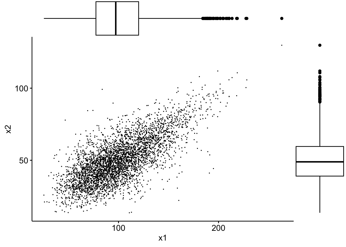
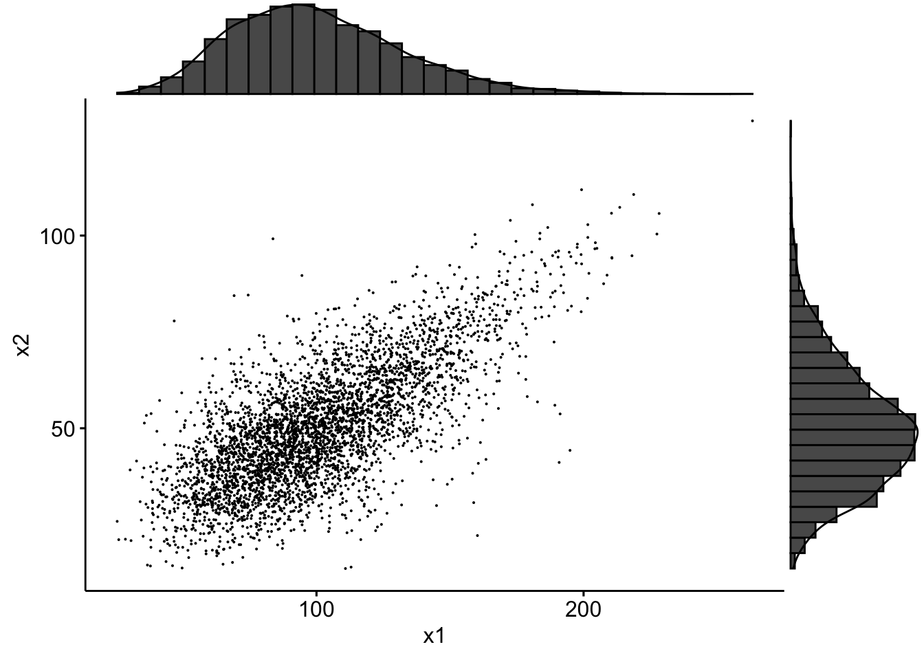
If we use the packages ggplot2, ggpubr and ggExtra one can superimpose density plots:
data <- tibble(x1 = Simul.x[, 1], x2 = Simul.x[, 2])
sp <- ggscatter(data, x = "x1", y = "x2", size = 0.05)
ggMarginal(sp, type = "density")

… or boxplots:
sp2 <- ggscatter(data, x = "x1", y = "x2", size = 0.05)
ggMarginal(sp2, type = "boxplot")
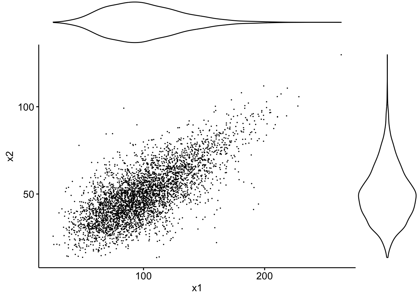
… or violin plots:
sp3 <- ggscatter(data, x = "x1", y = "x2", size = 0.05)
ggMarginal(sp3, type = "violin")
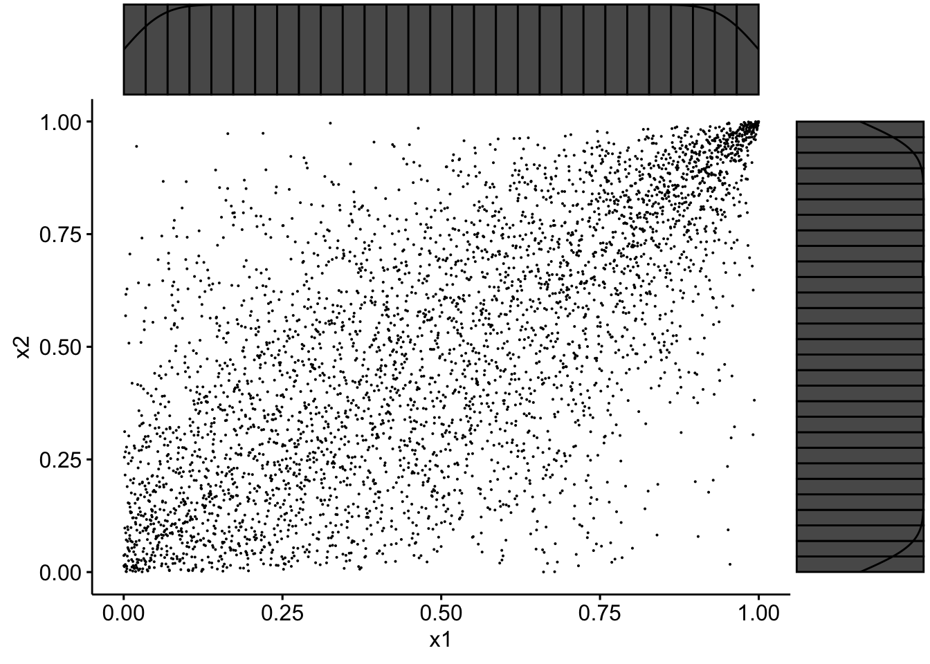
… or densigram plots:
sp4 <- ggscatter(data, x = "x1", y = "x2", size = 0.05)
ggMarginal(sp4, type = "densigram")
## Warning: The dot-dot notation (`..density..`) was deprecated in ggplot2 3.4.0.
## ℹ Please use `after_stat(density)` instead.
## ℹ The deprecated feature was likely used in the ggExtra package.
##   Please report the issue at
##   <https://github.com/daattali/ggExtra/issues>.
## This warning is displayed once every 8 hours.
## Call `lifecycle::last_lifecycle_warnings()` to see where this warning
## was generated.
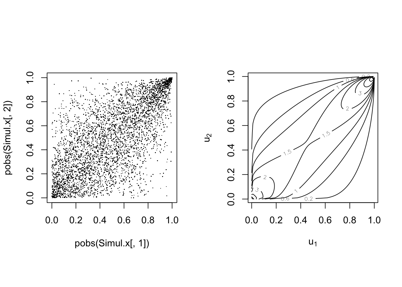
par(mfrow = c(1, 2), pty = "s")
plot(pobs(Simul.x[, 1]), pobs(Simul.x[, 2]), pch = ".")
plot(cop, type = "contour", margins = "unif")
data2 <- tibble(x1 = pobs(Simul.x[, 1]), x2 = pobs(Simul.x[,
  2]))
sp3 <- ggscatter(data2, x = "x1", y = "x2", size = 0.05)
ggMarginal(sp3, type = "densigram")
Ranks have uniform margins as expected.
\(\adv\) Fitting bivariate copulas
#
\(\adv\) Using R
#
The
VineCopula package offers many functions for fitting copulas:
BiCopKDE: A kernel density estimate of the copula density is visualised.BiCopSelect: Estimates the parameters of a bivariate copula for a set of families and selects the best fitting model (using either AIC or BIC). Returns an object of classBiCop.BiCopEst: Estimates parameters of a bivariate copula with a prespecified family. Returns an object of classBiCop. Estimation can be done by- maximum likelihood (method = “mle”) or
- inversion of the empirical Kendall’s tau (method = “itau”, only available for one-parameter families).
BiCopGofTest: Goodness-of-Fit tests for bivariate copulas.
\(\adv\) Case study with VineCopula: SUVA data
#
\(\adv\) Kernel density
#
BiCopKDE(pobs(SUVAcom[, 1]), pobs(SUVAcom[, 2]))
BiCopKDE(pobs(SUVAcom[, 1]), pobs(SUVAcom[, 2]), margins = "unif")
\(\adv\) Fitting
#
SUVAselect <- BiCopSelect(pobs(SUVAcom[, 1]), pobs(SUVAcom[,
  2]), selectioncrit = "BIC")
summary(SUVAselect)
## Family
## ------
## No:    10
## Name:  BB8
##
## Parameter(s)
## ------------
## par:  3.08
## par2: 0.99
## Dependence measures
## -------------------
## Kendall's tau:    0.52 (empirical = 0.52, p value < 0.01)
## Upper TD:         0
## Lower TD:         0
##
## Fit statistics
## --------------
## logLik:  488.99
## AIC:    -973.98
## BIC:    -964
For comparison:
SUVAsurvClayton <- BiCopEst(pobs(SUVAcom[, 1]), pobs(SUVAcom[,
  2]), family = 13)
summary(SUVAsurvClayton)
## Family
## ------
## No:    13
## Name:  Survival Clayton
##
## Parameter(s)
## ------------
## par:  2.07
##
## Dependence measures
## -------------------
## Kendall's tau:    0.51 (empirical = 0.52, p value < 0.01)
## Upper TD:         0.72
## Lower TD:         0
##
## Fit statistics
## --------------
## logLik:  478.14
## AIC:    -954.28
## BIC:    -949.29
\(\adv\) Further GOF
#
White’s test:
BiCopGofTest(pobs(SUVAcom[, 1]), pobs(SUVAcom[, 2]), SUVAselect)
## Error in BiCopGofTest(pobs(SUVAcom[, 1]), pobs(SUVAcom[, 2]), SUVAselect): The goodness-of-fit test based on White's information matrix equality is not implemented for the BB copulas.
BiCopGofTest(pobs(SUVAcom[, 1]), pobs(SUVAcom[, 2]), SUVAsurvClayton)
## $statistic
##          [,1]
## [1,] 1.343252
##
## $p.value
## [1] 0.26
We cannot perform the test on the BB8 copula (R informs us that The goodness-of-fit test based on White's information matrix equality is not implemented for the BB copulas.), but also cannot reject the null on the Survival Clayton.
BiCopGofTest(pobs(SUVAcom[, 1]), pobs(SUVAcom[, 2]), SUVAselect,
  method = "kendall")
## $p.value.CvM
## [1] 0.21
##
## $p.value.KS
## [1] 0.24
##
## $statistic.CvM
## [1] 0.08458458
##
## $statistic.KS
## [1] 0.738938
BiCopGofTest(pobs(SUVAcom[, 1]), pobs(SUVAcom[, 2]), SUVAsurvClayton,
  method = "kendall")
## $p.value.CvM
## [1] 0.34
##
## $p.value.KS
## [1] 0.23
##
## $statistic.CvM
## [1] 0.08144334
##
## $statistic.KS
## [1] 0.7731786
par(mfrow = c(1, 2), pty = "s")
BiCopKDE(pobs(SUVAcom[, 1]), pobs(SUVAcom[, 2]), margins = "unif")
plot(SUVAselect, type = "contour", margins = "unif")
par(mfrow = c(1, 2), pty = "s")
BiCopKDE(pobs(SUVAcom[, 1]), pobs(SUVAcom[, 2]), margins = "unif")
plot(SUVAsurvClayton, type = "contour", margins = "unif")
\(\adv\) Case study with censoring: ISO data
#
\(\adv\) Insurance company losses and expenses
#
- Data consists of 1,500 general liability claims.
- Provided by the Insurance Services Office, Inc.
\(X_{1}\)is the loss, or amount of claims paid.\(X_{2}\)are the ALAE, or Allocated Loss Adjustment Expenses.- Policy contains policy limits, and hence, censoring.
\(\delta\)is the indicator for censoring so that the observed data consists of
$$\left( x_{1i},x_{2i},\delta _{i}\right) \text{ for }i=1,2,...,1500.$$
We will fit this data mostly “by hand” for transparency (and since we need to allow for censoring). R codes are provided separately.
Loss.ALAE <- read_csv("LossData-FV.csv")
## Rows: 1500 Columns: 4
## ── Column specification ──────────────────────────────────────────────
## Delimiter: ","
## dbl (4): LOSS, ALAE, LIMIT, CENSOR
##
## ℹ Use `spec()` to retrieve the full column specification for this data.
## ℹ Specify the column types or set `show_col_types = FALSE` to quiet this message.
as_tibble(Loss.ALAE)
## # A tibble: 1,500 × 4
##     LOSS  ALAE   LIMIT CENSOR
##    <dbl> <dbl>   <dbl>  <dbl>
##  1    10  3806  500000      0
##  2    24  5658 1000000      0
##  3    45   321 1000000      0
##  4    51   305  500000      0
##  5    60   758  500000      0
##  6    74  8768 2000000      0
##  7    75  1805  500000      0
##  8    78    78  500000      0
##  9    87 46534  500000      0
## 10   100   489  300000      0
## # ℹ 1,490 more rows
\(\adv\) Summary statistics of data
#
| Loss | ALAE | Policy Limit | Loss (Uncensored) | Loss (Censored) | |
|---|---|---|---|---|---|
| Number | 1,500 | 1,500 | 1,352 | 1,466 | 34 |
| Mean | 41,208 | 12,588 | 559,098 | 37,110 | 217,491 |
| Median | 12,000 | 5,471 | 500,000 | 11,048 | 100,000 |
| Std Deviation | 102,748 | 28,146 | 418,649 | 92,513 | 258,205 |
| Minimum | 10 | 15 | 5,000 | 10 | 5,000 |
| Maximum | 2,173,595 | 501,863 | 7,500,000 | 2,173,595 | 1,000,000 |
| 25th quantile | 4,000 | 2,333 | 300,000 | 3,750 | 50,000 |
| 75th quantile | 35,000 | 12,577 | 1,000,000 | 32,000 | 300,000 |
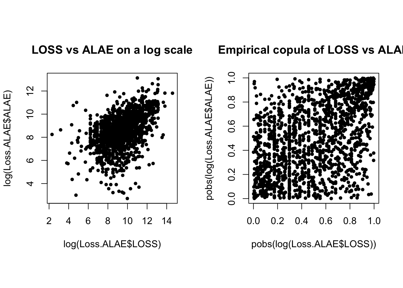
\(\adv\) loss vs ALAE
#
par(mfrow = c(1, 2), pty = "s")
plot(log(Loss.ALAE$LOSS), log(Loss.ALAE$ALAE), main = "LOSS vs ALAE on a log scale",
  pch = 20)
plot(pobs(log(Loss.ALAE$LOSS)), pobs(log(Loss.ALAE$ALAE)), main = "Empirical copula of LOSS vs ALAE",
  pch = 20)
par(mfrow = c(1, 2), pty = "s")
BiCopKDE(pobs(log(Loss.ALAE$LOSS)), pobs(log(Loss.ALAE$ALAE)))
BiCopKDE(pobs(log(Loss.ALAE$LOSS)), pobs(log(Loss.ALAE$ALAE)),
  margins = "unif")
\(\adv\) Maximum likelihood estimation
#
- Case 1: loss variable is not censored, i.e.
\(\delta =0.\)
$$f\left( x_{1},x_{2}\right) =f_{1}\left( x_{1}\right) f_{2}\left( x_{2}\right) C_{12}\left( F_{1}\left( x_{1}\right) ,F_{2}\left( x_{2}\right) \right)$$
where \(C_{12}(u_1,u_2)=\frac{\partial C(u_1,u_2)}{\partial u_1\partial u_2}\).
- Case 2: loss variable is censored, i.e.
\(\delta =1.\)
$$\begin{array}{rcl} \frac{\partial }{\partial x_{2}}P\left( X_{1}>x_{1},X_{2}\leq x_{2}\right) &=&\frac{\partial }{\partial x_{2}}\left[ F_{2}\left( x_{2}\right) -F\left(x_{1},x_{2}\right) \right] \\\\ &=&f_{2}\left( x_{2}\right) -\frac{\partial}{\partial x_2}F\left( x_{1},x_{2}\right) \\\\ &=&f_{2}\left( x_{2}\right) \left[ 1-C_2\left( F_{1}\left(x_{1}\right) ,F_{2}\left( x_{2}\right) \right) \right] \end{array}$$
where \(C_i(u_1,u_2)=\frac{\partial C(u_1,u_2)}{\partial u_i}\).
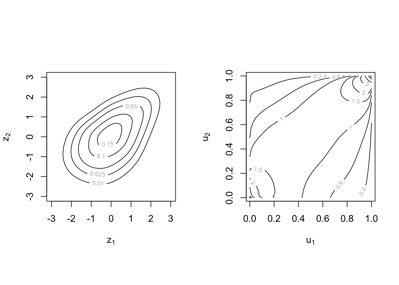
\(\adv\) Choice of marginals and copulas
#
- Pareto marginals:
\(F_{k}\left( x_{k}\right) =1-\left( \frac{\lambda_{k}}{\lambda _{k}+x_{k}}\right) ^{\theta _{k}}\)for\(k=1,2.\)and\(x>0\). - For the copulas, several candidates were used:
\(\adv\) Parameter estimates
#
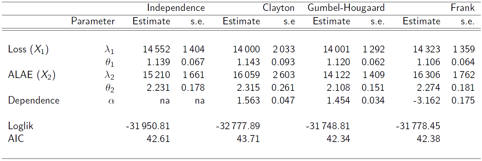
\(\adv\) AIC criterion
#
-
Akaike Information Criterion (AIC)
-
In the absence of a better way to choosing/selecting a copula model, one may use the AIC criterion defined by
$$\text{AIC}=\left( -2\ell +2m\right)/n$$where\(\ell\)is the value of maximised log-likelihood,\(m\)is the number of parameters estimated, and\(n\)is the sample size. -
Lower AIC generally is preferred.
\(\adv\) Summary
#
To find the distribution of the sum of dependent random variables with copulas (one approach):
- Fit marginals independently
- Describe/fit dependence with a copula (roughly)
- Get a sense of data (scatterplots, dependence measures)
- Choose candidate copulas
- For each candidate, estimate parameters via MLE
- Choose a copula based on nll(highest) or AIC(lowest)
- If focusing on the sum, one might do simulations to look at the distributions of aggregates, and how they compare with the original data.
Coefficients of tail dependence #
Motivation #
- In insurance and investment applications it is the large outcomes (losses) that particularly tend to occur together, whereas small claims tend to be fairly independent
- This is one of the reasons why tails (especially right tails) tend to be fatter in financial applications.
- A good understanding of tail behaviour is hence very important.
- It is possible to derive tail properties due to dependence from a copula model.
- The indicator we are considering here is the coefficient of tail dependence.
- Tail dependence can take values between 0 (no dependence) and 1 (full dependence).
VineCopula::BiCopPar2TailDepcomputes the theoretical tail dependence coefficients for copulas of theBiCopfamily.
Coefficient of lower tail dependence #
The coefficient of lower tail dependence is defined as
$$\lambda_L=\lim_{u\rightarrow 0^+} \Pr\left[ X_1 \le F_{X_1}^{-1}(u) \left| X_2\le F_{X_2}^{-1}(u)\right.\right] = \lim_{u\rightarrow 0^+} \frac{C(u,u)}{u}.$$
Examples (note the extensive use of de l’Hospital rule):
$$\begin{array}{rcl} \lambda_L^{\text{ind}}&=&\displaystyle\lim_{u\rightarrow 0^+} \frac{u\cdot u}{u} =\lim_{u\rightarrow 0^+} u = 0 \\ \lambda_L^{\text{Clayton}}&=&\displaystyle\lim_{u\rightarrow 0^+} \frac{\left( 2 u^{-\theta}-1\right)^{-1/\theta}}{u} = \displaystyle \lim_{u\rightarrow 0^+} \frac{\left( 2 -u^\theta\right)^{-1/\theta}u}{u}\\ &=&\displaystyle\lim_{u\rightarrow 0^+} \left( 2 -u^\theta\right)^{-1/\theta}=2^{-1/\theta} = \left(\frac{1}{2}\right)^{\frac{1}{\theta}} \end{array}$$
The lower tail of the Clayton copula is comprehensive in that
it allows for tail coefficients of 0 (as \(\theta \rightarrow 0\) ) to 1 (as \(\theta \rightarrow \infty\) ).
Coefficient of upper tail dependence #
The coefficient of upper tail dependence is defined similarly but using the survival copula, which yields
$$\begin{array}{rcl} \lambda_U&=&\lim_{u\rightarrow 1^-} \Pr\left[ X_1 \ge F_{X_1}^{-1}(u) \left| X_2\ge F_{X_2}^{-1}(u)\right.\right] \\ &=& \displaystyle \lim_{u\rightarrow 1^-} \frac{\overline{C}(1-u,1-u)}{1-u} = \lim_{u\rightarrow 0^+} \frac{\overline{C}(u,u)}{u}. \end{array}$$
Note \(\overline{C}(u,u)=2u-1+C(1-u,1-u).\) Examples:
$$\begin{array}{rcl} \lambda_U^{\text{ind}}&=&\displaystyle\lim_{u\rightarrow 1^-} \frac{1-2u+u^2}{1-u} = \lim_{u\rightarrow 1^-} 1-u =0 \\ \lambda_U^{\text{Frank}}&=&\displaystyle\lim_{u\rightarrow 1^-} \frac{1-2u+1/\theta\left[\log(e^{2\theta u}-2e^{\theta u}+e^\theta)-\log(e^\theta-1)\right]}{1-u} \\ &=&\displaystyle\lim_{u\rightarrow 1^-} \frac{-2+1/\theta\cdot(2\theta e^{2\theta u}-2\theta e^{\theta u})/(e^{2\theta u}-2e^{\theta u}+e^\theta)}{-1} \\ &=&0 \end{array}$$
References #
Avanzi, Benjamin, Luke C. Cassar, and Bernard Wong. 2011. “Modelling Dependence in Insurance Claims Processes with Lévy Copulas.” ASTIN Bulletin 41 (2): 575–609.
Kurowicka, D., and H. Joe. 2011. Dependence Modeling Vine Copula Handbook.
Nelsen, R. B. 1999. An Introduction to Copulas. Springer.
Sklar, A. 1959. “Fonctions de Répartition à $n$ Dimensions Et Leurs Marges.” Publications de l’Institut de Statistique de l’Université de Paris 8: 229–31.
Vigen, Tyler. 2015. “Spurious Correlations (Last Accessed on 18 March 2015 on http://www.tylervigen.com).”
Wikipedia. 2020. “Copula: Probability Theory.” https://www.wikiwand.com/en/Copula_(probability_theory).