Algorithms for compound distributions #
Preliminary: Discretisation #
- In the algorithms considered in this module (and in real life..!), severity distributions are discrete.
- In Module 3 we discussed how to fit parametric distributions to real data, but these were continuous (which often allows to define a whole df easily with just a few parameters).
- This is not a restriction as the distribution of
\(Y\)can easily be discretised to an arbirary level of precision. - Different methods have different properties and are used for different purposes.
- A number of those methods are easily implemented, thanks to the function
discretiseofactuar.
There are three (four) methods, all covered by the R function actuar::discretise:
- Mass dispersal (
method="rounding"): a first try to allocate weights in a rather `unbiased’ way. In this case, the true cdf passes through the midpoints of the discretisation intervals. - Unbiased (
method="unbiased"): this method matches the first moment of the discretised and the true distributions. - Lower (
method="lower") and Upper (method="upper") bounds, which sandwich the correct distribution between two arbitrarily close bounds. Here the idea is to intentionally underestimate and overestimate the distribution. However, the gap in-between can be chosen to be arbitrarily small.
in discretise, we will also need to specify:
step\(=h\): a currency span (say, $10 or $100)from\(=0\): the left limit of discretisation (we set this to 0 here, a natural bound for positive claims distributions)to\(=mh\): the right limit of discretisationcdf: the distribution to discretise (in cumulative, cdf form—thepfoofunction)
Method of rounding (mass dispersal) #
- apportion the probability mass to a finite set of points
\(0, h, 2h, \ldots, mh\) - if the range of
\(X\)is not finite,\(m\)has to be chosen in order to have a good representation of the right tail - the span
\(h\)should be carefully chosen as to be relatively small compared to the mean (beware of units!) - Let
\(g_j\)be the probability mass placed at\(jh\),\(j=0,1,\ldots,m\). We have
$$\begin{array}{rcl} g_0 &=& G\left( h/2 \right) \\ g_j &=& G\left( jh + h/2\right)-G\left( jh - h/2\right),\quad g=1,2,\ldots,m-1 \\ g_m &=& 1-G\left(mh-h/2\right) \end{array}$$
such that \(\sum_{j=0}^m g_j=1\).
(Note that if \(G\) is mixed and a mass happens to be at an interval threshold, it is customary—for conservativeness—to allocate it to the next
interval, so that \(G\) would be understood as càglàd here.)
Unbiased method #
- Let
\(g_j\)be the probability mass placed at\(jh\),\(j=0,1,\ldots,m\). We have
$$\begin{array}{rcl} g_0 &=& 1 - E[\min(X,h)]/h \\ g_j &=& (2 E[\min(X,j)]-E[\min(X,j-h)]-E[\min(X,j+h)])/h,\\ &&j=1,2,\ldots,m-1 \\ g_m &=& (E[\min(X,m)]-E[\min(X,m-h)])/h-(1-G(m)) \end{array}$$
such that \(\sum_{j=0}^m g_j=G(m)\).
- Note that in this case the parameter
levmust be specified. This is an expression that computes the limited expected value of the distribution corresponding tocdf. This is readily available inactuarfor many distributions.
Method of lower and upper bounds #
Define:
$$G((k+1)d)-G(kd) = \left\{ \begin{array}{ll} \Pr[Y_1^+=(k+1)d] \equiv g_{k+1}^+ & \text{(shifted to the right)} \\ \Pr[Y_1^-=k d] \equiv g_{k}^- & \text{(shifted to the left)} \end{array} \right.$$
Note that from a stochastic dominance point of view
\(Y_1^+\)(method="lower") overestimates (is larger than)\(Y_1\), whereas\(Y_1^-\)(method="upper") underestimates (is smaller than)\(Y_1\).
This means that we can sandwich the true distribution:
$$\Pr[Y^- > y] \le \Pr[Y>y] \le \Pr[Y^+ > y], \text{ or}$$
$$\Pr[Y^- \le y] \ge \Pr[Y\le y] \ge \Pr[Y^+ \le y] \Longleftrightarrow G^+(y)\le G(y) \le G^-(y).$$
This can be the best option, especially for patchwork distributions;
see Example 4.12 in Wuthrich (2023).
Examples #
Let us discretise
stp <- 5
final <- 80
# these are pmf's
gamma.discr.round <- discretise(pgamma(x, 2, 0.1), from = 0,
  to = final, step = stp, method = "rounding")
gamma.discr.unbia <- discretise(pgamma(x, 2, 0.1), from = 0,
  to = final, step = stp, method = "unbiased", lev = levgamma(x,
    2, 0.1))
gamma.discr.lower <- discretise(pgamma(x, 2, 0.1), from = 0,
  to = final, step = stp, method = "lower")
gamma.discr.upper <- discretise(pgamma(x, 2, 0.1), from = 0,
  to = final, step = stp, method = "upper")
length(gamma.discr.round)
## [1] 16
length(gamma.discr.unbia)
## [1] 17
length(gamma.discr.lower)
## [1] 17
length(gamma.discr.upper)
## [1] 16
Note the different lengths (either \(m\) or \(m+1\)), although they all start with \(g_0\).
Furthermore, the masses don’t add up to 1 necessarily:
sum(gamma.discr.round)
## [1] 0.996231
pgamma(final - stp/2, 2, 0.1)
## [1] 0.996231
sum(gamma.discr.unbia)
## [1] 0.9969808
sum(gamma.discr.lower)
## [1] 0.9969808
sum(gamma.discr.upper)
## [1] 0.9969808
pgamma(final, 2, 0.1)
## [1] 0.9969808
This is because the algorithm does not adjust for the tail:
roundinghas\(g_m = G(m+h/2)-G(m-h/2)\)rather than\(g_m = 1-G(m-h/2)\)so that\(1-G(m+h/2)\)is missing.unbiasedhas that correction\(-(1-G(m))\)(due to the fact that this mass does not correspond to this interval) which is then missing.lowerhas\(g_0=0\)and then the mass\(G(m)\)is apportioned to the end of the\(m\)intervals.\(1-G(m)\)remains unallocated.upperhas its first allocation from\(G(m)\)at 0, so has one less mass in the vector.\(1-G(m)\)remains unallocated.
In practice one would choose \(m\) sufficiently large so that these are issues are not present. If they are, then, an adjustment might be necessary, and rounding becomes the most natural one to use (just add the missing mass at \(g_m\) as per the definition above).
# getting df's
gamma.discr.round.df <- cumsum(gamma.discr.round)
gamma.discr.unbia.df <- cumsum(gamma.discr.unbia)
gamma.discr.lower.df <- cumsum(gamma.discr.lower)
gamma.discr.upper.df <- cumsum(gamma.discr.upper)
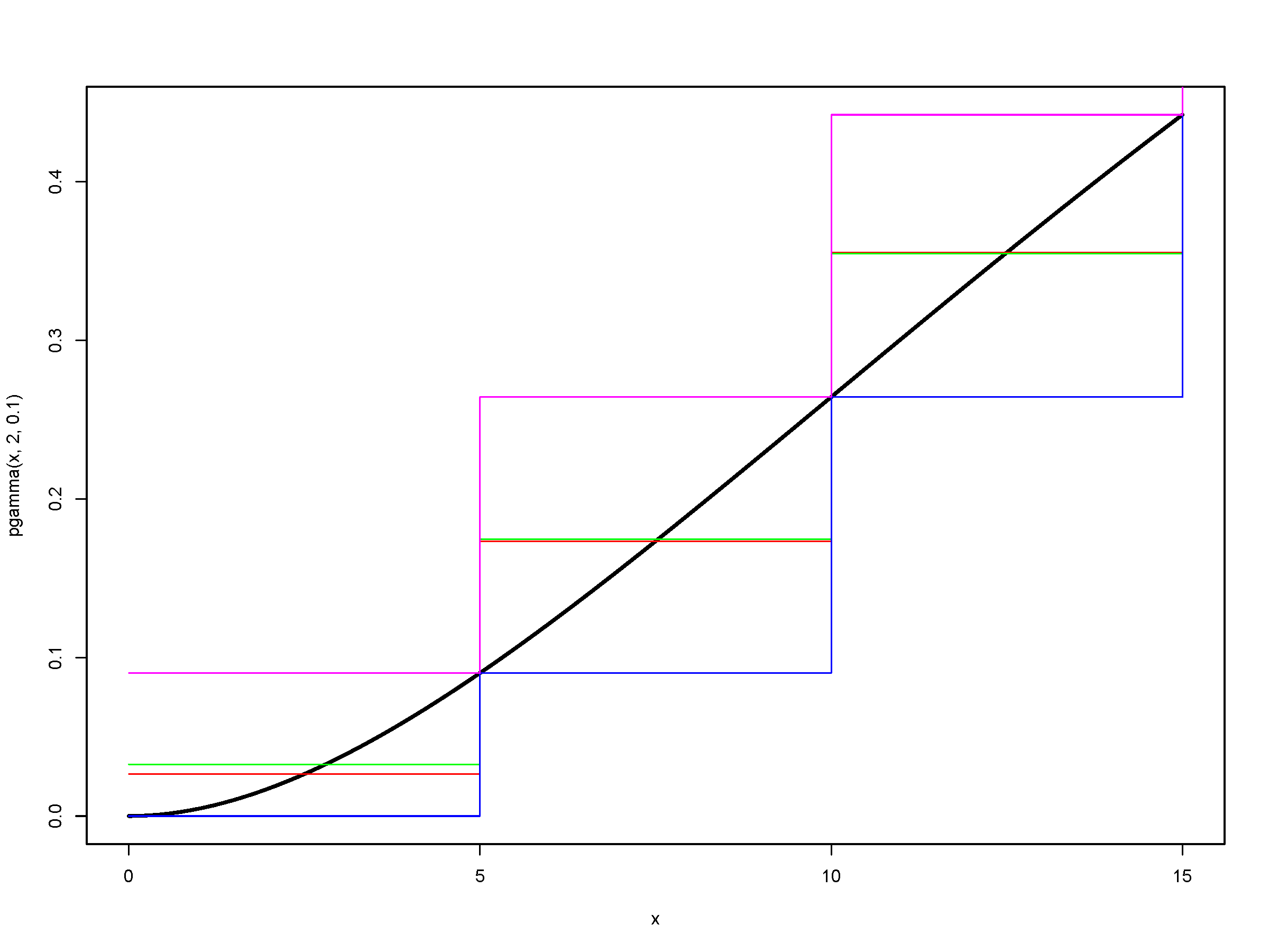
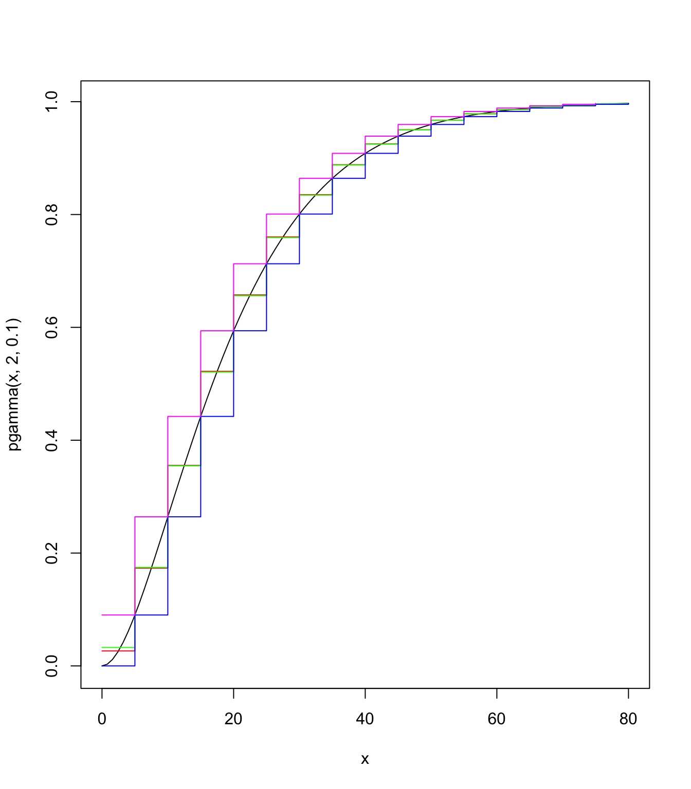
# comparing discretisation techniques
curve(pgamma(x, 2, 0.1), from = 0, to = final)
lines((0:(final/stp - 1)) * stp, gamma.discr.round.df, type = "s",
pch = 20, col = "red")
lines((0:(final/stp)) * stp, gamma.discr.unbia.df, type = "s",
pch = 20, col = "green")
lines((0:(final/stp)) * stp, gamma.discr.lower.df, type = "s",
pch = 20, col = "blue")
lines((0:(final/stp - 1)) * stp, gamma.discr.upper.df, type = "s",
pch = 20, col = "magenta")
Panjer’s recursion algorithm (MW 4.2.1) #
- The remarkable property of the
\((a,b)\)class of (frequency) distributions allows us to develop a recursive method to get the distribution of\(S\)for discrete\(Y\)’s. - When
\(Y\)is continuous, simply discretise its cdf first. - The algorithm is very stable when
\(N\)is Poisson and Negative Binomial, but less stable when\(N\)is Binomial.
Let \(S\) have a compound distribution on \(Y\), where the following are mutually independent:
\(N\)belongs to the\((a,b)\)class of distributions;\(Y\)are identically distributed, non-negative and discrete.
We have then
$$f_{S}\left( s\right) =\frac{1}{1-a g_0 }\sum_{j=1}^{s}\left( a+b\frac{j}{s}\right) g_j f_{S}\left( s-j\right),\quad s=1,2,\ldots,$$
with starting value
$$f_{S}\left( 0\right) =\left\{ \begin{array}{ll} \Pr\left[ N=0\right] , & \text{if }g_0 =0 \\ M_{N}\left[ \ln g_0 \right] , & \text{if }g_0 >0. \end{array} \right.$$
Note that if \(g_y=0\) for \(y>y_{\text{max}}\) then the upper bound of the sum can be reduced to \(\min(s,y_{\text{max}}).\)
Panjer’s recursion in R #
Panjer’s recursion can be performed using the aggregateDist function using the method="recursive".
- The frequency distribution can be any of the
\((a,b,0)\)or\((a,b,1)\)class of distributions (that is, with arbitrary masses at 0). - The severity distribution must be discrete on
\(0,1,\ldots,m\)for some monetary unit.
Important parameters include:
model.freq: name of the distribution (e.g.="poisson")model.sev: df of the discrete (-ised) distribution of\(Y\)x.scale: value of an amount 1 in the severity model (monetary unit)maxit: maximum number of iterations, which often needs to be increased (if it is too small then the df of\(S\)does not reach 1, leading to an error message)
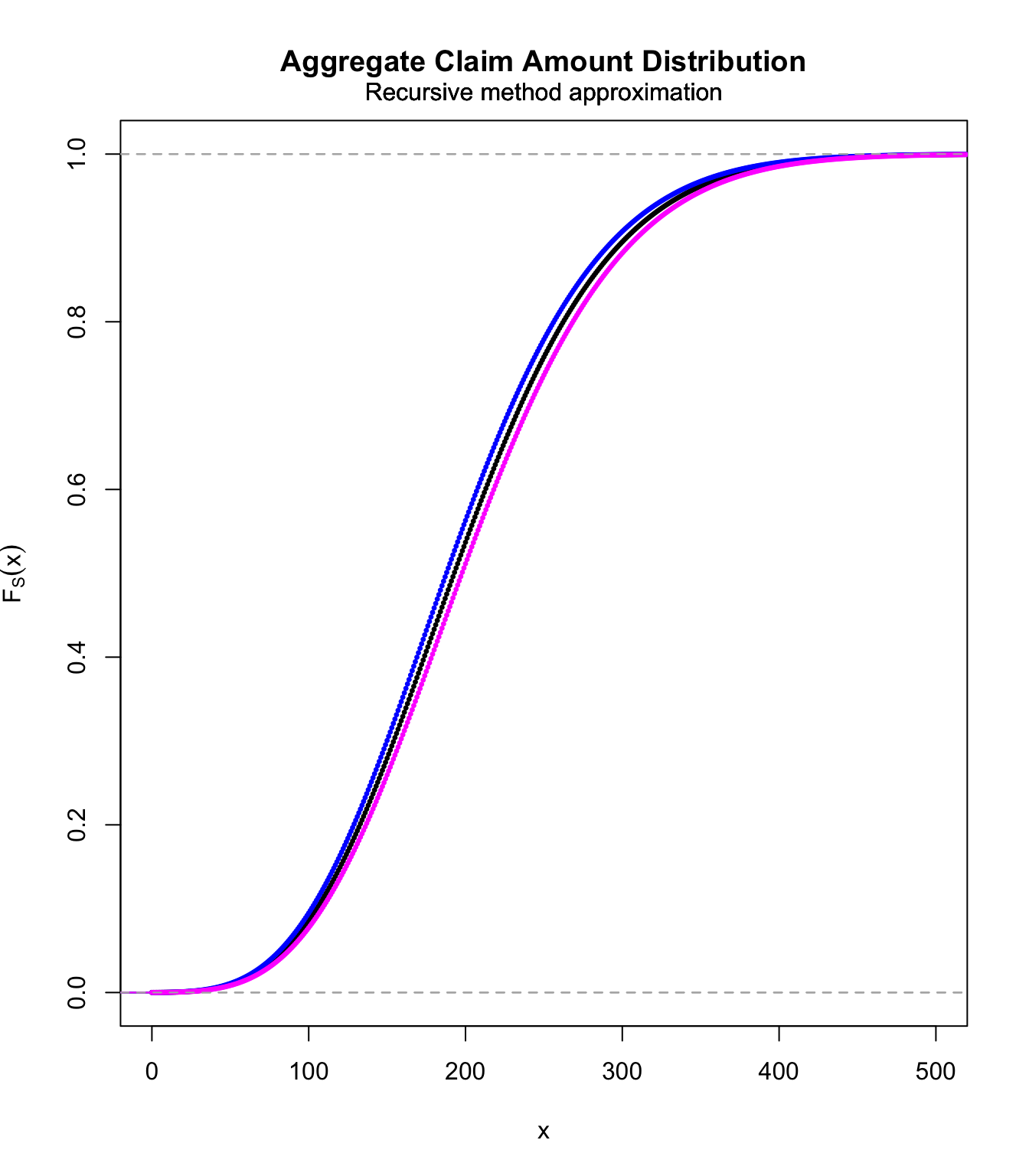
Example #
We want to calculate the distribution of
$$S=\sum_{i=1}^N Y_i,$$
where \(N\sim\text{Poi}(10)\) and \(Y_1\sim\text{gamma}(2,0.1)\).
stp <- 1
final <- 200
# these are pmf's
gamma.discr.unbia <- discretise(pgamma(x, 2, 0.1), from = 0,
  to = final, step = stp, method = "unbiased", lev = levgamma(x,
    2, 0.1))
gamma.discr.lower <- discretise(pgamma(x, 2, 0.1), from = 0,
  to = final, step = stp, method = "lower")
gamma.discr.upper <- discretise(pgamma(x, 2, 0.1), from = 0,
  to = final, step = stp, method = "upper")
S.unbia.cdf <- aggregateDist(method = "recursive", model.freq = "poisson",
  lambda = 10, model.sev = gamma.discr.unbia, x.scale = stp,
  maxit = 1000)
S.lower.cdf <- aggregateDist(method = "recursive", model.freq = "poisson",
  lambda = 10, model.sev = gamma.discr.lower, x.scale = stp,
  maxit = 1000)
S.upper.cdf <- aggregateDist(method = "recursive", model.freq = "poisson",
  lambda = 10, model.sev = gamma.discr.upper, x.scale = stp,
  maxit = 1000)
plot(S.unbia.cdf, pch = 20, xlim = c(0, 500), col = "black",
  cex = 0.5)
lines(S.upper.cdf, pch = 20, col = "blue", cex = 0.5)
lines(S.lower.cdf, pch = 20, col = "magenta", cex = 0.5)
Panjer’s recursion for compound Poisson #
If \(S\sim\text{compound Poisson}(\lambda,g_x)\) the algorithm reduces to
$$f_{S}\left( s\right) =\frac{\lambda}{s}\sum_{j=1}^{s} \, j\,g_j f_{S}\left( s-j\right) \text{.}$$
with starting value
$$f_{S}\left( 0\right) =e^{\lambda(g_0-1)}$$
(whether \(g_0\) is positive or not).
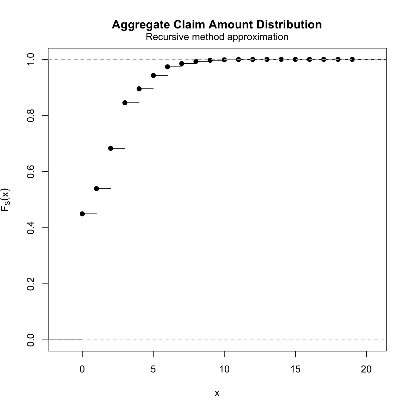
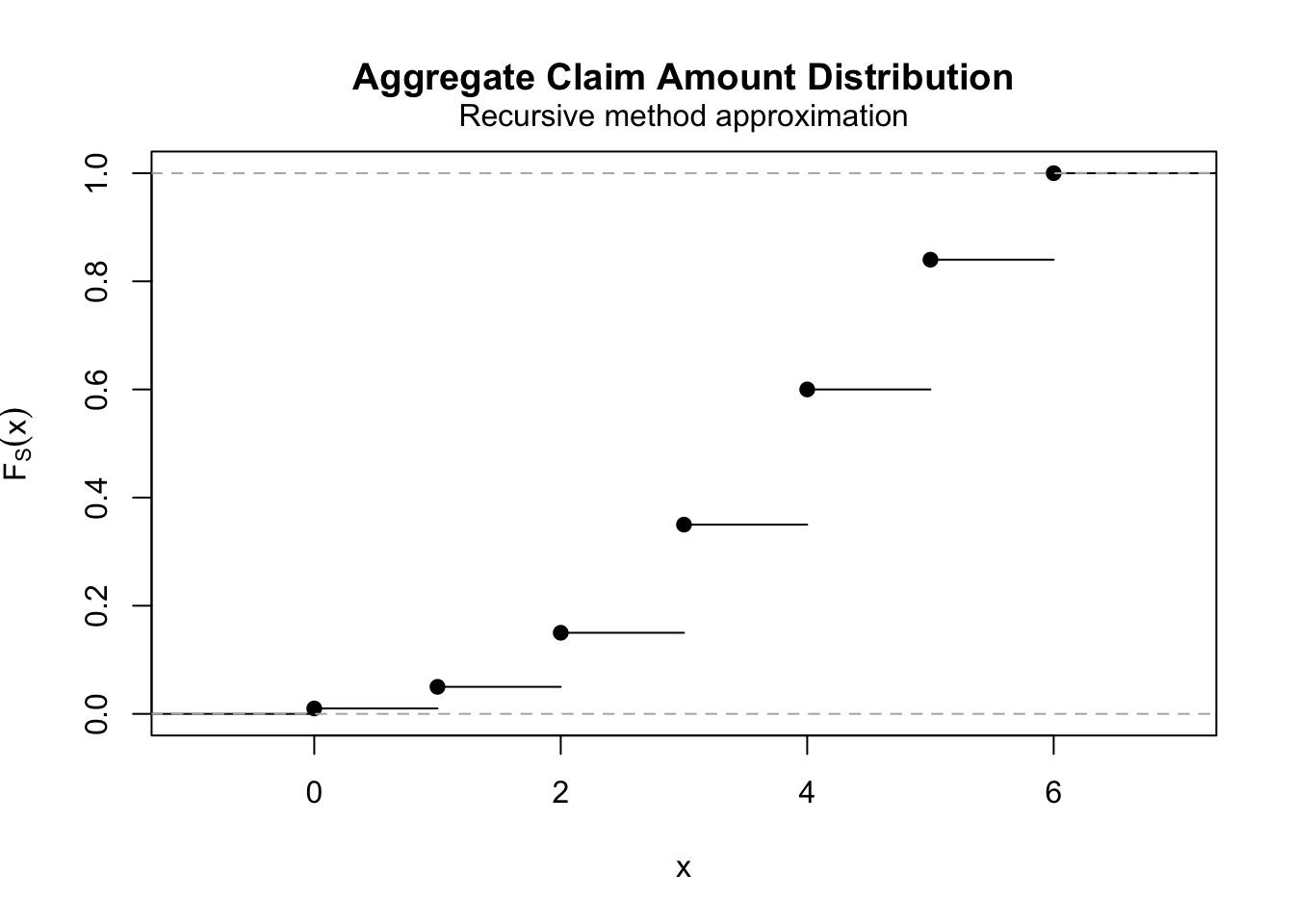
Example A 12.4.2 (recomputed) #
Effectively, the recursion formula boils down to
$$f_{S}\left( s\right) =\frac{1}{s}\left[ 0.2f_{S}\left( s-1\right)+0.6f_{S}\left( s-2\right) +0.9f_{S}\left( s-3\right) \right], \;\; (\text{for }s>2)$$
with starting value
$$f_{S}\left( 0\right) =\Pr\left[ N=0\right]=e^{-0.8}=0.44933.$$
We have then
$$\begin{array}{rcl} f_{S}\left( 1\right) &=& 0.2f_{S}\left( 0\right) =0.2e^{-0.8}=0.089866 \\ f_{S}\left( 2\right) &=&\frac{1}{2}\left[ 0.2f_{S}\left( 1\right)+0.6f_{S}\left( 0\right) \right] =0.32e^{-0.8}=0.14379 \\ f_{S}\left( 3\right) &=&\frac{1}{3}\left[ 0.2f_{S}\left( 2\right)+0.6f_{S}\left( 1\right) +0.9f_{S}\left( 0\right) \right]=0.3613e^{-0.8}=0.16236 \\ && etc \ldots \end{array}$$
fs <- aggregateDist(method = "recursive", model.freq = "poisson",
  lambda = 0.8, model.sev = c(0, 0.25, 0.375, 0.375), x.scale = 1)
diff(fs)[1:4]
## [1] 0.44932896 0.08986579 0.14378527 0.16235753
plot(fs)
\(\adv\) de Pril’s recursion algorithm
#
As a corollary, a recursion algorithm can be developed for the \(n\)-th convolution of a non-negative and discrete random variable \(Y\) with positive mass of probability at 0. Let \(g_k\) be its pmf.
First let us rewrite
$$\begin{array}{rcl} M_Y(t)&=&\sum_{k=0}^\infty g_k e^{tk}=g_0+\sum_{k=1}^\infty g_k e^{tk} \\ &=&g_0 + [1-g_0]\sum_{k=1}^\infty \frac{g_k}{1-g_0} e^{tk} \\ &=& q + p m_{\widetilde{Y}}(t). \end{array}$$
where
\(q=g_0\),\(p=1-g_0\), and- the pmf of
\(\widetilde{Y}\)is:\(\widetilde{g}_0=0\),\(\widetilde{g}_k=\frac{g_k}{1-g_0}\),\(k=1,2,\cdots\).
Thus
$$E\left[e^{t(Y_1+\ldots+Y_n)}\right]=\left(M_Y(t)\right)^n=\left(q + p m_{\widetilde{Y}}(t)\right)^n,$$
which means that the \(n\)-th convolution of \(Y\) is compound Binomial with parameters \((m=n,p=1-g_0,\widetilde{G}(y))\), a member of the \((a,b)\) class with
$$\begin{array}{rcl} a&=&-\frac{p}{1-p} \\ &=& -\frac{1-g_0}{g_0}, \\ b&=&\frac{(m+1)p}{1-p} \\ &=& \frac{(n+1)(1-g_0)}{g_0}. \end{array}$$
Applying Panjer’s algorithm yields
with
$$g^{*n}_0=g_0^n.$$
Note that the \(g_j\)’s are indeed the original ones.
Numerical example #
Let \(g_k=(1+k)/10\), \(k=0,1,2\) and \(3\). We have
$$g^{*2}_k=\sum_{j=1}^{\min(k,3)}\left[3\frac{j}{k}-1\right](1+j)g^{*2}_{k-j}\:\text{ with }\:g^{*2}_0=[g_0]^2$$
$$\begin{array}{rcl} g^{*2}_0&=&(0.1)^2=0.01\\ g^{*2}_1&=&[3/1-1] \cdot 2 \cdot 0.01=0.04 \\ g^{*2}_2&=&[3/2-1] \cdot 2 \cdot 0.04+[6/2-1] \cdot 3 \cdot 0.01=0.10 \\ g^{*2}_3&=&[3/3-1] \cdot 2 \cdot 0.10+[6/3-1] \cdot 3 \cdot 0.04+[9/3-1] \cdot 4 \cdot 0.01=0.20 \\ g^{*2}_4&=&[3/4-1] \cdot 2 \cdot 0.20+[6/4-1] \cdot 3 \cdot 0.10+[9/4-1] \cdot 4 \cdot 0.04=0.25 \\ g^{*2}_5&=&[3/5-1] \cdot 2 \cdot 0.25+[6/5-1] \cdot 3 \cdot 0.20+[9/5-1] \cdot 4 \cdot 0.10=0.24 \\ g^{*2}_6&=&[3/6-1] \cdot 2 \cdot 0.24+[6/6-1] \cdot 3 \cdot 0.25+[9/6-1] \cdot 4 \cdot 0.20=0.16 \end{array}$$
brute force convolution:
pmf <- c(1/10, 2/10, 3/10, 4/10)
range <- length(pmf)
range2 <- (range - 1) * 2 + 1
pmf <- c(pmf, rep(0, (range2 - range)))
ps2.conv <- c()
for (i in 1:range2) {
  ps2.conv <- c(ps2.conv, sum(pmf[1:i] * pmf[i:1]))
}
ps2.conv
## [1] 0.01 0.04 0.10 0.20 0.25 0.24 0.16
Using de Pril’s algorithm
ps2 <- aggregateDist(method = "recursive", model.freq = "binomial",
  size = 2, prob = 1 - 1/10, model.sev = c(0, 2/10, 3/10, 4/10)/(1 -
    1/10), x.scale = 1, xlim = c(0, 6))
diff(ps2)
## [1] 0.01 0.04 0.10 0.20 0.25 0.24 0.16
plot(ps2)
\(\adv\) Fast Fourier Transform
#
Not covered this year.
Approximations #
Possible motivations:
- It is not possible to compute the distribution of
\(S\):- no detailed data is available except for the moments of
\(S\) - technical issues (impossible to fit a tractable model to data)
- no detailed data is available except for the moments of
- The risk of having a sophisticated—but wrong—model is too high
- Only limited data is available to fit the model
- It may be argued that the approximation is very accurate
- A quick approximation is needed.
- A higher level of accuracy is not required (does not justify the resources necessary to calculate an exact probability)
Note: let \(\varsigma_S\equiv\gamma_1\) and \(\gamma_2(S)\equiv\gamma_2\) in this section.
Approximations assuming a symmetrical distribution #
The Normal approximation (MW 4.1.1) #
- The Central Limit Theorem suggests that
$$\begin{array}{rcl} \Pr\left[ S\leq s\right] &=& =\Pr\left[ \frac{S-E[S] }{\sqrt{Var(S)} }\leq \frac{s-E[S] }{\sqrt{Var(S)} }\right] \\ &\approx &\Pr\left[ Z\leq \frac{s-E[S] }{\sqrt{Var(S)} }\right]=\Phi \left( \frac{s-E[S] }{\sqrt{Var(S)} }\right) , \end{array}$$
where \(Z\) is a standard Normal random variable and where \(\Phi \left( \cdot \right)\) denotes its cdf
- The classical CLT approximation holds for a fixed number of claims. Here, we typically have a random number of claims.
- Assuming
\(S\sim\text{CompPoi}(\lambda v,G)\), Theorem 4.1 of Wuthrich (2023) states that $$ \frac{S-\lambda v E[Y]}{\sqrt{\lambda v E[Y^2]}} \Longrightarrow \mathcal{N}(0,1)\quad \text{as }v\rightarrow \infty.$$ - This leads to the approximation
$$\Pr[S\le s] = \Pr \left[\frac{S-\lambda v E[Y]}{\sqrt{\lambda v E[Y^2]}} \le \frac{s-\lambda v E[Y]}{\sqrt{\lambda v E[Y^2]}}\right] \approx \Phi\left(\frac{s-\lambda v E[Y]}{\sqrt{\lambda v E[Y^2]}}\right).$$ - Note that this holds only when
\(G\)has a finite second moment, which suggests that this should be used only for\(S_{\text{sc}}\).
Note that this approximation performs poorly
- individual model: for small
\(n\)(CLT not effective) - collective model: for small
\(\lambda v\)(compound Poisson) and small\(r\)(compound negative binomial) - for highly skewed distributions
\(\adv\) Normal Power
#
Two levels:
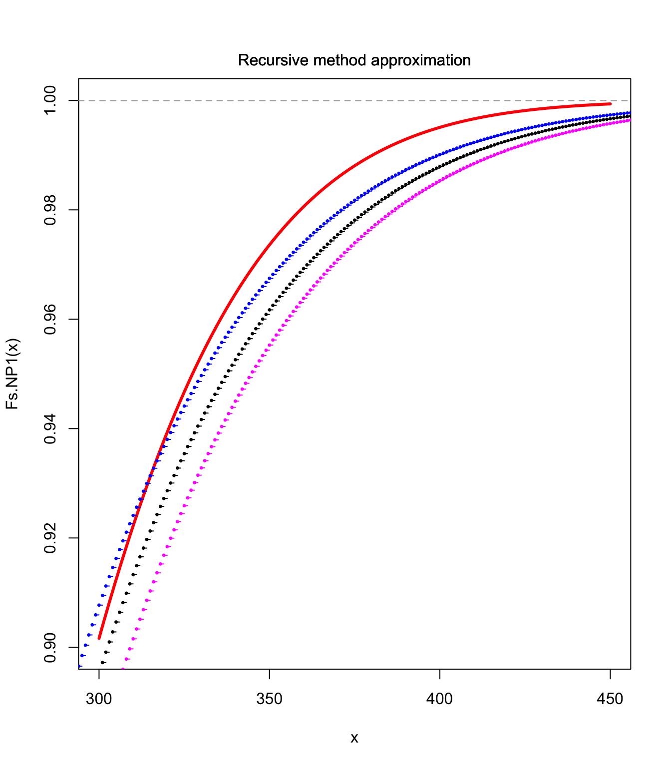
- NP1: this is the CLT approximation
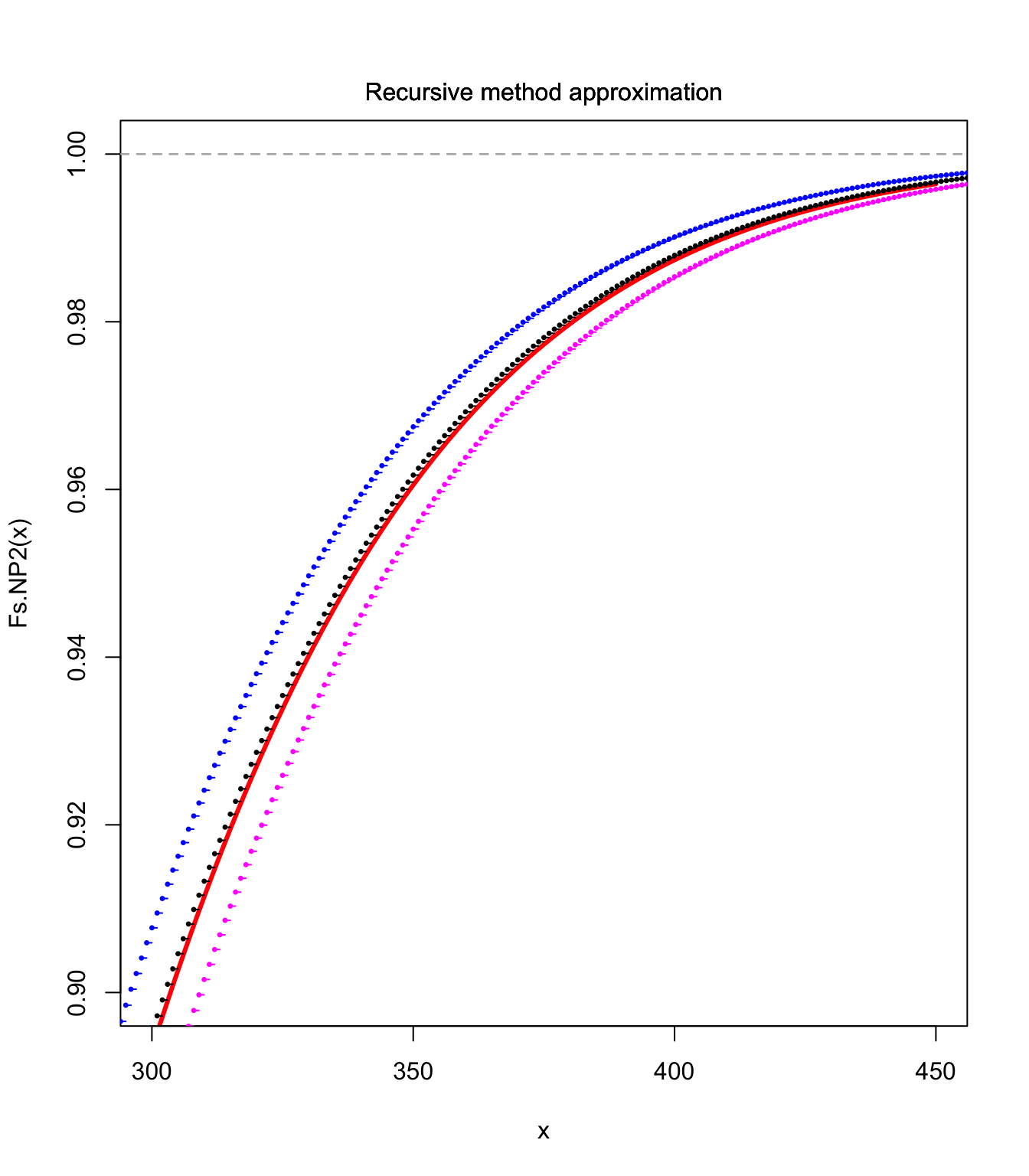
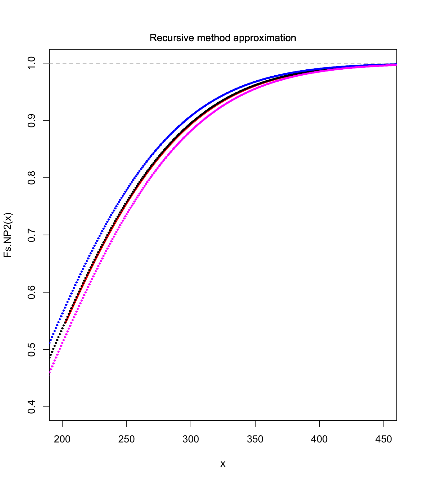
- NP2: the same idea, but with a correction taking the skewness into account. We have
$$\Pr\left[ \frac{S-E[S] }{\sqrt{Var(S)} }\leq s\right] \approx \Phi \left( z\right)$$with$$s(z)=z+\frac{\gamma_1}{6} \left(z^{2}-1\right)\quad\text{ or }\quad z(s)=\sqrt{\frac{9}{\gamma_1 ^{2}}+\frac{6s}{\gamma_1 }+1}-\frac{3}{\gamma_1 }$$NP2 is effective for\(S>E[S]+\sqrt{Var(S)}\).
- NP1 and NP2 approximations are available with the
aggregateDistfunction - For instance here use on a compound Poisson random variable with gamma distributed claims:
gamma <- 2
c <- 0.1
lambda <- 10
moments <- c(lambda * gamma/c, lambda * (gamma/c^2 + (gamma/c)^2),
  gamma * (gamma + 1) * (gamma + 2)/c^3/lambda^(1/2)/(gamma/c^2 +
    (gamma/c)^2)^(3/2))
Fs.NP1 <- aggregateDist("normal", moments = moments)
curve(Fs.NP1, xlim = c(300, 450), ylim = c(0.9, 1), col = "red",
  lwd = 3)
lines(S.unbia.cdf, pch = 20, cex = 0.5)
lines(S.upper.cdf, pch = 20, col = "blue", cex = 0.5)
lines(S.lower.cdf, pch = 20, col = "magenta", cex = 0.5)
Fs.NP2 <- aggregateDist("npower", moments = moments)
curve(Fs.NP2, xlim = c(300, 450), ylim = c(0.9, 1), col = "red",
  lwd = 3)
lines(S.unbia.cdf, pch = 20, cex = 0.5)
lines(S.upper.cdf, pch = 20, col = "blue", cex = 0.5)
lines(S.lower.cdf, pch = 20, col = "magenta", cex = 0.5)
curve(Fs.NP2, xlim = c(200, 450), ylim = c(0.4, 1), col = "red",
  lwd = 3)
lines(S.unbia.cdf, pch = 20, cex = 0.5)
lines(S.upper.cdf, pch = 20, col = "blue", cex = 0.5)
lines(S.lower.cdf, pch = 20, col = "magenta", cex = 0.5)
Approximations using a skewed distribution #
The translated gamma and LN approximations (MW 4.1.2) #
Idea: Rather than correcting the CLT approximation, we use here a distribution that is naturally (positively) skewed, and use the third moment (skewness), which will be fitted thanks to a translation of the distribution (a third parameter to match the third moment).
We have then
$$X = k+Z, \text{ where }Z\sim \left\{ \begin{array}{l} \Gamma(\gamma,c), \text{ or}\\\text{LN}(\mu,\sigma^2)\end{array}\right. .$$
Then match expected value, variance and skewness.
Note: \(k\) appears only in the expected value. It allows to shift the distribution without affecting its scale (and central moments).
As an example, fitting a translated gamma \((k,\gamma,c)\) to a compPois$(\lambda v,G(y))$ \(S\equiv X\) boils down to solving
$$\begin{array}{rcl} E[S]=\lambda v E[Y] &=& k+\gamma/c; \\ Var(S)=\lambda v E[Y^2]&=& \gamma/c^2; \\ \varsigma_S=\frac{E[Y^3]}{(\lambda v)^{1/2} E[Y^2]^{3/2}} &=& 2\gamma^{-1/2}; \end{array}$$
such that
$$\begin{array}{rcl} \gamma &=& \left(\frac{2(\lambda v)^{1/2} E[Y^2]^{3/2}}{E[Y^3]}\right)^2; \\ c &=& \left(\frac{\gamma}{\lambda v E[Y^2]}\right)^{1/2}; \\ k &=& \lambda v E[Y] - \frac{\gamma}{c}. \end{array}$$
Properties of the translated gamma approximation:
- If
\(\gamma\rightarrow\infty\),\(c\rightarrow\infty\)and\(k\rightarrow -\infty\)such that$$E[S]=k+\frac{\gamma}{c}=\mu\text{ (constant)}\quad\text{and}\quad \frac{\gamma}{c^2}=\sigma^2\text{ (constant)}$$then the translated gamma converges to the Normal\((\mu,\sigma^2)\)distribution. In this sense, this approximation is a generalisation of the CLT approximation. - The distribution of a compound binomial random variable approaches the gamma distribution if the expected number of claims is large and the claim amount distribution has relatively small dispersion (see Theorem 12.A.1 in the Appendix of Chapter 12 of Bowers et al. (1997)).
- This approximation should be used for distributions with a positive skewness only.
# matching moments:
gamma <- (2/moments[3])^2
c <- (gamma/moments[2])^(1/2)
k <- moments[1] - gamma/c
# check:
c(gamma/c + k, moments[1])
## [1] 200 200
c((gamma/c^2), moments[2])
## [1] 6000 6000
c(2 * gamma^(-1/2), moments[3])
## [1] 0.5163978 0.5163978
plot(200:450, pgamma(200:450 - k, shape = gamma, rate = c), xlim = c(200,
  450), ylim = c(0.4, 1), col = "red", lwd = 3, type = "l",
  xlab = c(""))
lines(S.unbia.cdf, pch = 20, cex = 0.5)
lines(S.upper.cdf, pch = 20, col = "blue", cex = 0.5)
lines(S.lower.cdf, pch = 20, col = "magenta", cex = 0.5)
![]()
curve(Fs.NP2, xlim = c(320, 390), ylim = c(0.93, 0.98), col = "red",
  lwd = 1)
lines(300:450, pgamma(300:450 - k, shape = gamma, rate = c),
  col = "green", lwd = 1, type = "l")
lines(S.unbia.cdf, pch = 20, cex = 0.5)
lines(S.upper.cdf, pch = 20, col = "blue", cex = 0.5)
lines(S.lower.cdf, pch = 20, col = "magenta", cex = 0.5)
![]()
When approximating a discrete distribution with a continuous one, a half-integer discontinuity correction needs to be applied. Let \(S\sim\text{Poisson}(\lambda=16)\). Possible approximations are
- Translated gamma with
\(\gamma=64\),\(c=2\)and\(k=-16\). - CLT with
\(E[S]=Var(S)=16\)
Results are below:
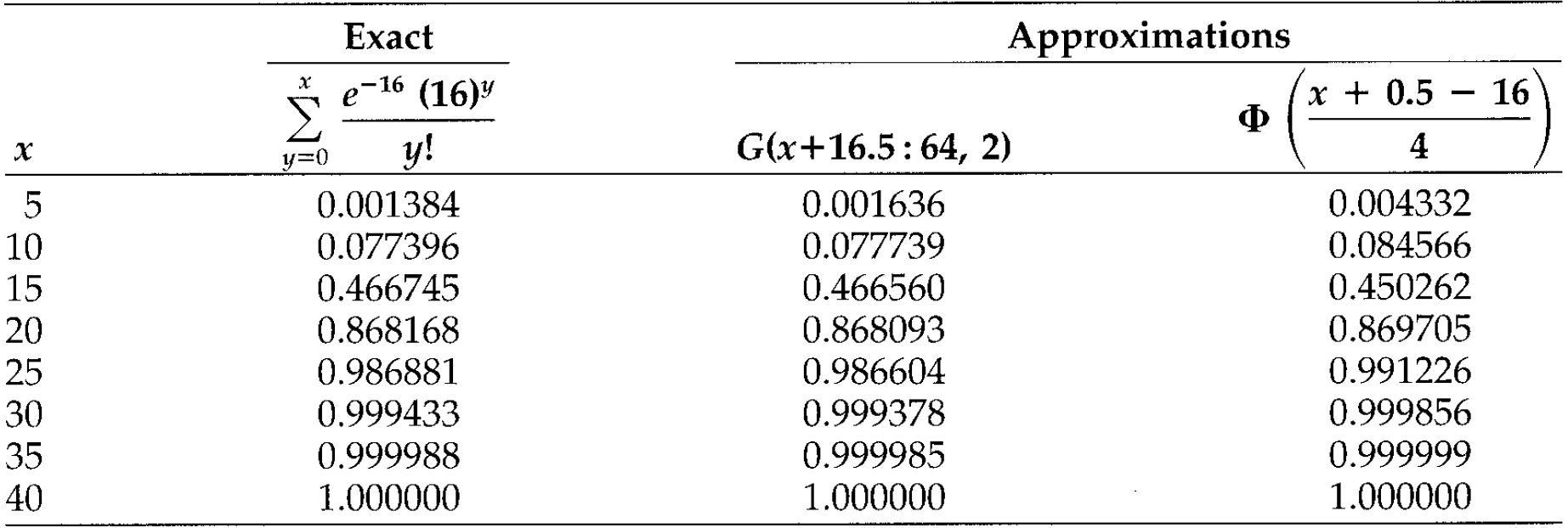
Note that the discretisation techniques take this into account.
\(\adv\) Edgeworth’s approximation (MW 4.1.3)
#
Let
$$\Phi^{(k)}(x)=\frac{d^k}{dx^k}\Phi(x).$$
We have then (each term improves the accuracy)
$$\Pr\left[ \frac{S-E[S] }{\sqrt{Var(S)} }\leq z\right] \approx\Phi(z)-\frac{\gamma_1}{6}\Phi^{(3)}(z)+\frac{\gamma_2}{24}\Phi^{(4)}(z)+\frac{\gamma_1^2}{72}\Phi^{(6)}(z).$$
Note
$$\begin{array}{rcl} \Phi^{(1)}(x)&=&\varphi(x)=\frac{1}{\sqrt{2\pi}}e^{-\frac{1}{2}x^2} \\ \Phi^{(2)}(x)&=&-x\varphi(x) \\ \Phi^{(3)}(x)&=&(x^2-1)\varphi(x) \\ & \text{etc} \ldots & \end{array}$$
\(\qquad\) Problem is: it sometimes leads to negative probabilities…
\(\adv\) Approximating the Individual Model with the Collective Model
#
Mainly motivated by the properties of compound distributions, in particular the compound Poisson:
- aggregation
- recursive methods
We want to approximate \(\widetilde{S}\) (IRM) by \(S\) (CRM):
$$\widetilde{S}=\sum_{i=1}^{n}I_{i}b_{i}\approx S=\sum_{i=1}^{n}N_{i}b_{i},$$
where \(N_i\sim\text{Poisson}(\lambda_i)\) represents the number of claims of amount \(b_i\). \(S\) is then compound Poisson with parameters
$$\lambda =\sum_{i=1}^{n}\lambda _{i}\text{ \ and \ }P\left(x\right) =\sum_{i=1}^{n}\frac{\lambda _{i}}{\lambda }I_{\left[b_{i},\infty \right) }\left( x\right).$$
Two possible assumptions for \(\lambda_i\)
#
\(\lambda_i=E[I_i]=q_i\): the canonical collective model- expected number of claims of size
\(b_{i}\)will be the same between the two models - also implies equal expected claim numbers in both
\(\widetilde{S}\)and\(S\) - finally
$$\begin{array}{rcl} E\left( \widetilde{S}\right)=\sum_{i=1}^{n}q_{i}b_{i} &=&\lambda \sum_{i=1}^{n}\frac{q_{i}}{\lambda }b_{i}=E\left( S\right),\text{ but} \\ Var\left( \widetilde{S}\right) =\sum_{i=1}^{n}q_{i}\left(1-q_{i}\right) b_{i}^{2} & < & \sum_{i=1}^{n}q_{i}b_{i}^{2}=Var\left( S\right). \end{array}$$
- expected number of claims of size
\(\lambda_i=-\ln (1-q_i) >q_i\)\(\Pr[S=0]=\Pr[\widetilde{S}=0]\)
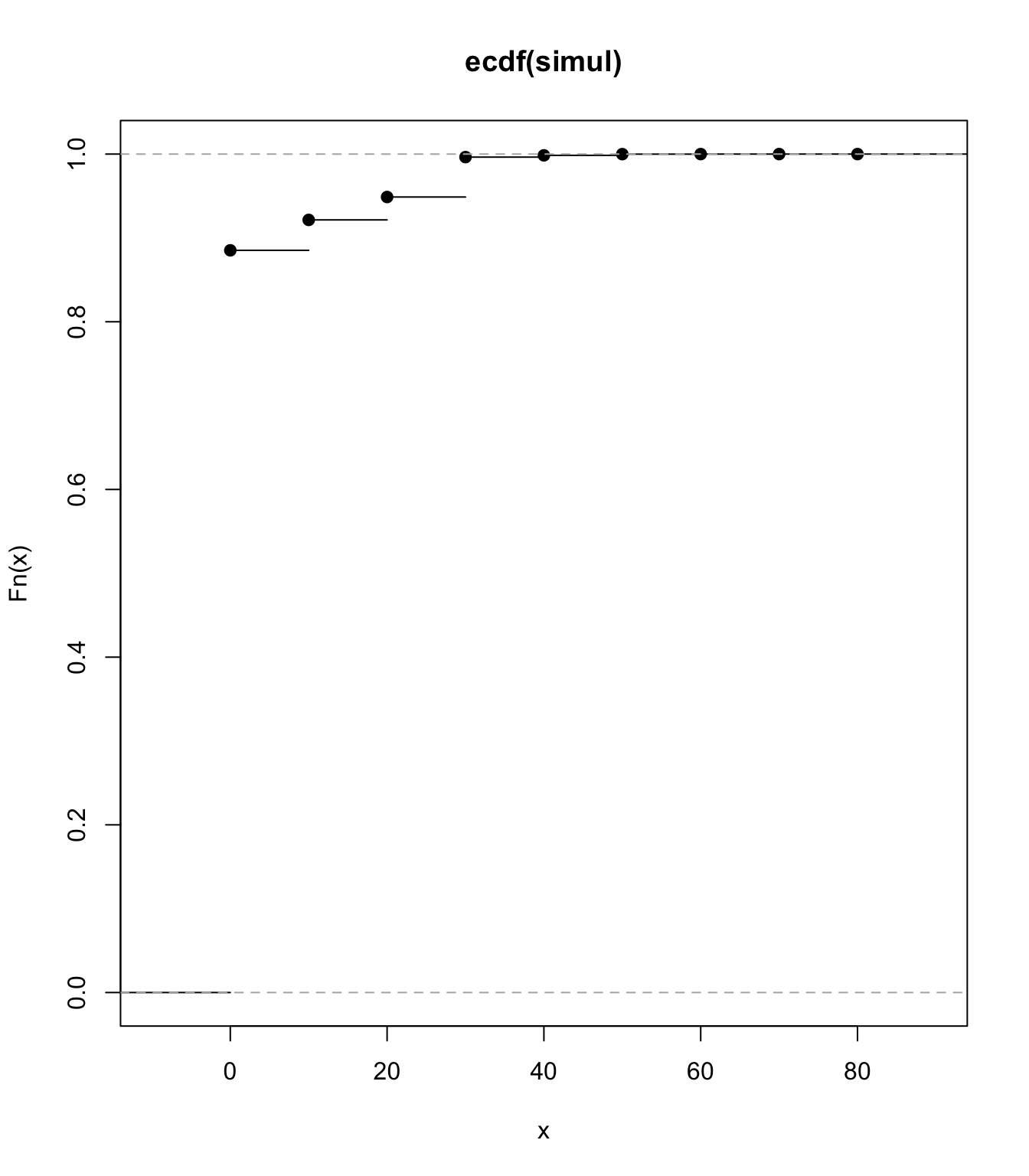
Example #
qi <- c(0.01, 0.02, 0.03, 0.01, 0.05)
bi <- c(10, 20, 10, 20, 30)
set.seed(10052021)
nsim <- 1e+07
simulated <- cbind(c(rbinom(nsim, 1, qi[1]) * bi[1]), c(rbinom(nsim,
  1, qi[2]) * bi[2]), c(rbinom(nsim, 1, qi[3]) * bi[3]), c(rbinom(nsim,
  1, qi[4]) * bi[4]), c(rbinom(nsim, 1, qi[5]) * bi[5]))
simul <- rowSums(simulated)
mean(simul)
## [1] 2.497127
plot(ecdf(simul))
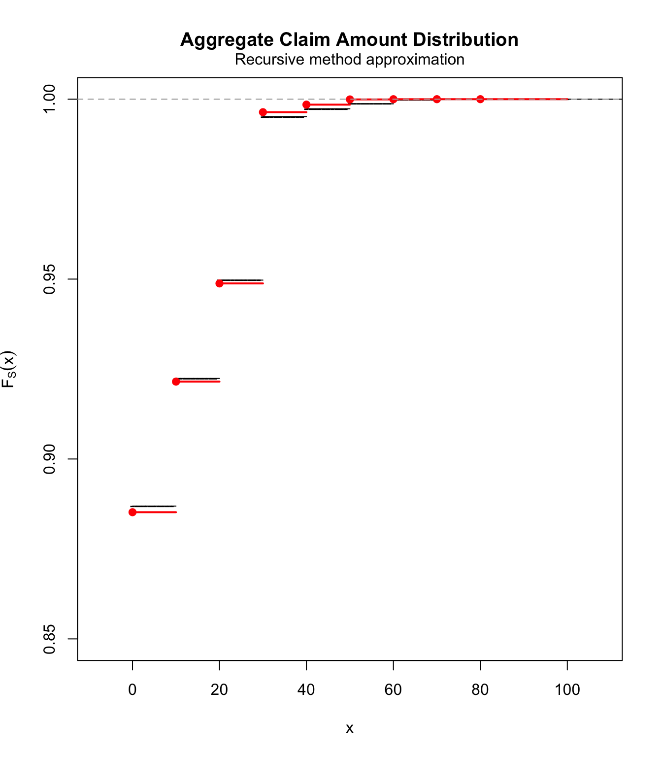
lambdai.1 <- qi
lambda.1 <- sum(lambdai.1)
pmf.1 <- c(rep(0, 10), (lambdai.1[1] + lambdai.1[3])/lambda.1,
  rep(0, 9), (lambdai.1[2] + lambdai.1[4])/lambda.1, rep(0,
    9), lambdai.1[5]/lambda.1)
fs.1 <- aggregateDist("recursive", model.freq = "poisson", model.sev = pmf.1,
  lambda = lambda.1)
plot(fs.1, ylim = c(0.85, 1), pch = "-")
lines(ecdf(simul), col = "red", lwd = 2)
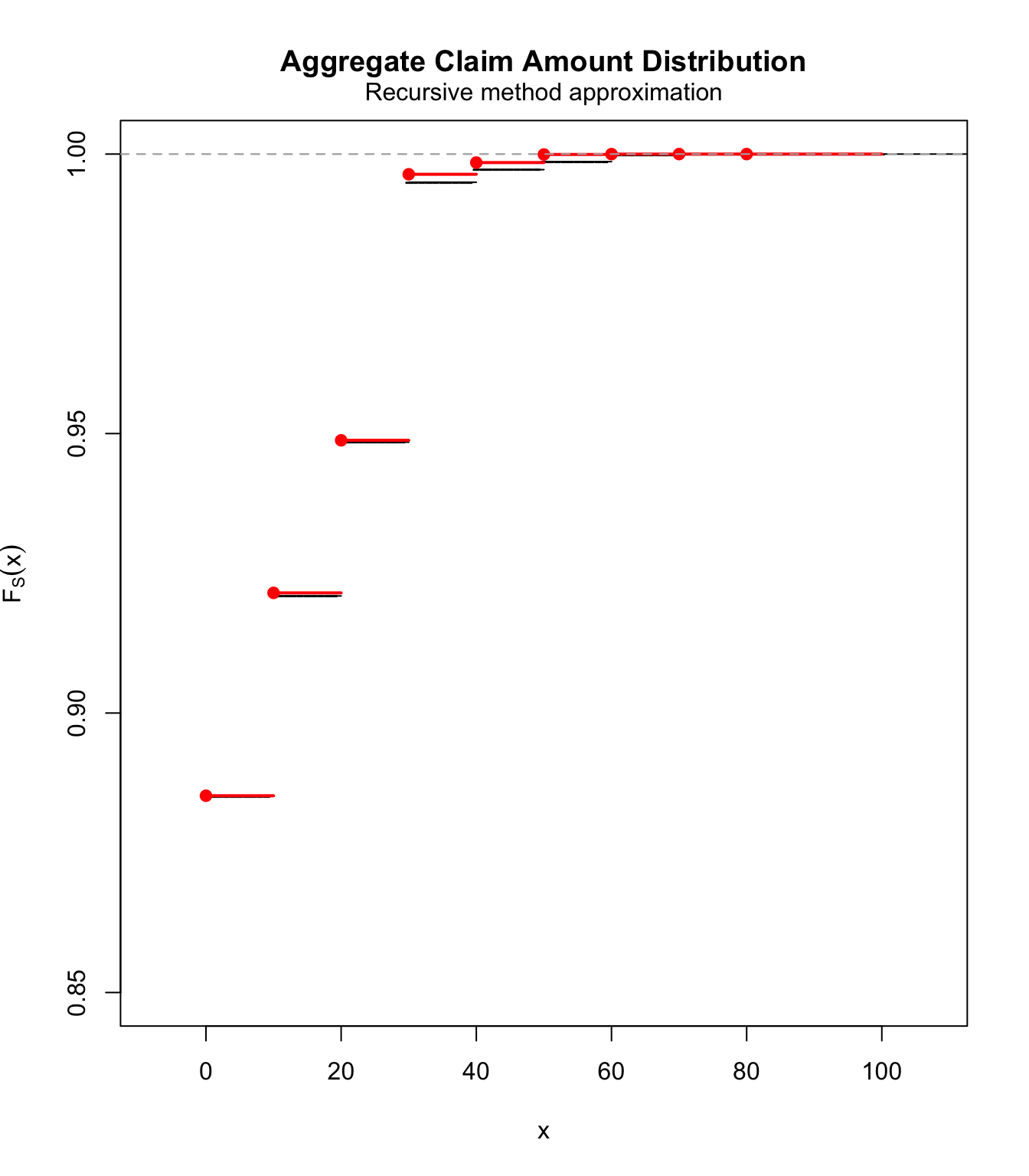
lambdai.2 <- -log(1 - qi)
lambda.2 <- sum(lambdai.2)
pmf.2 <- c(rep(0, 10), (lambdai.2[1] + lambdai.2[3])/lambda.2,
  rep(0, 9), (lambdai.2[2] + lambdai.2[4])/lambda.2, rep(0,
    9), lambdai.2[5]/lambda.2)
fs.2 <- aggregateDist("recursive", model.freq = "poisson", model.sev = pmf.2,
  lambda = lambda.2)
plot(fs.2, ylim = c(0.85, 1), pch = "-")
lines(ecdf(simul), col = "red", lwd = 2)
\(\adv\) Bringing it all together: SUVA case study
#
- We come back to the SUVA data; see Avanzi, Cassar, and Wong (2011).
- The right tail of the medical costs will be best modelled using an Extreme Value distribution (see Module 6), but this will result in a poor fit in the left tail.
- As a consequence we will fit the SUVA medical costs using two layers,
\(S_{\text{sc}}\)and\(S_{\text{lc}}\). If\(S\)is one medical cost claim (which can be scaled up easily), then$$S = S_{\text{sc}}+S_{\text{lc}}= \sum_{i=1}^{N_{\text{sc}}} X_{i,\text{sc}} + \sum_{j=1}^{N_{\text{lc}}} X_{j,\text{lc}},$$where\(N_{\text{sc}}\sim\text{Poi}(\lambda_{\text{sc}})\)and\(N_{\text{lc}}\sim\text{Poi}(\lambda_{\text{lc}})\), all mutually independent with the\(X_{\text{sc}}\)and\(X_{\text{lc}}\).
- The small claims layer can be tackled in different ways:
- use the empirical distribution for
\(X_{\text{sc}}\)and get the distribution of\(S_{\text{sc}}\)with Panjer. This is OK if the data is smooth enough and we don’t necessarily want the smoothing effect of a parametric distribution. - use an approximation such as translated gamma or normal power on
\(S_{\text{sc}}\). This has the potential of smoothing out a coarse empirical distribution.
- use the empirical distribution for
- The large claims layer fits
\(X_{\text{lc}}\)using EVT and then uses Panjer to get the distribution of\(S_{\text{lc}}\).- A threshold of $10,000 is chosen; see Module 6 for a justification.
Preliminaries #
Basic parameters:
M <- 10000
data.scale <- 100
Loading data:
SUVA <- read_excel("SUVA.xls")
as_tibble(SUVA)
## # A tibble: 2,326 × 2
##    medcosts dailyallow
##       <dbl>      <dbl>
##  1      407          0
##  2    12591      13742
##  3      269          0
##  4      142          0
##  5      175          0
##  6      298        839
##  7       47          0
##  8       59          0
##  9      191       7446
## 10      159          0
## # ℹ 2,316 more rows
Split claims #
Xsc <- SUVA$medcosts[SUVA$medcosts <= M]
Xsc <- Xsc[Xsc > 0]
Xlc <- SUVA$medcosts[SUVA$medcosts > M]
lambda.sc <- length(Xsc)/(length(Xsc) + length(Xlc))
lambda.lc <- length(Xlc)/(length(Xsc) + length(Xlc))
c(lambda.sc, lambda.lc)
## [1] 0.97109827 0.02890173
Modelling the small claims #
plotdist(Xsc)
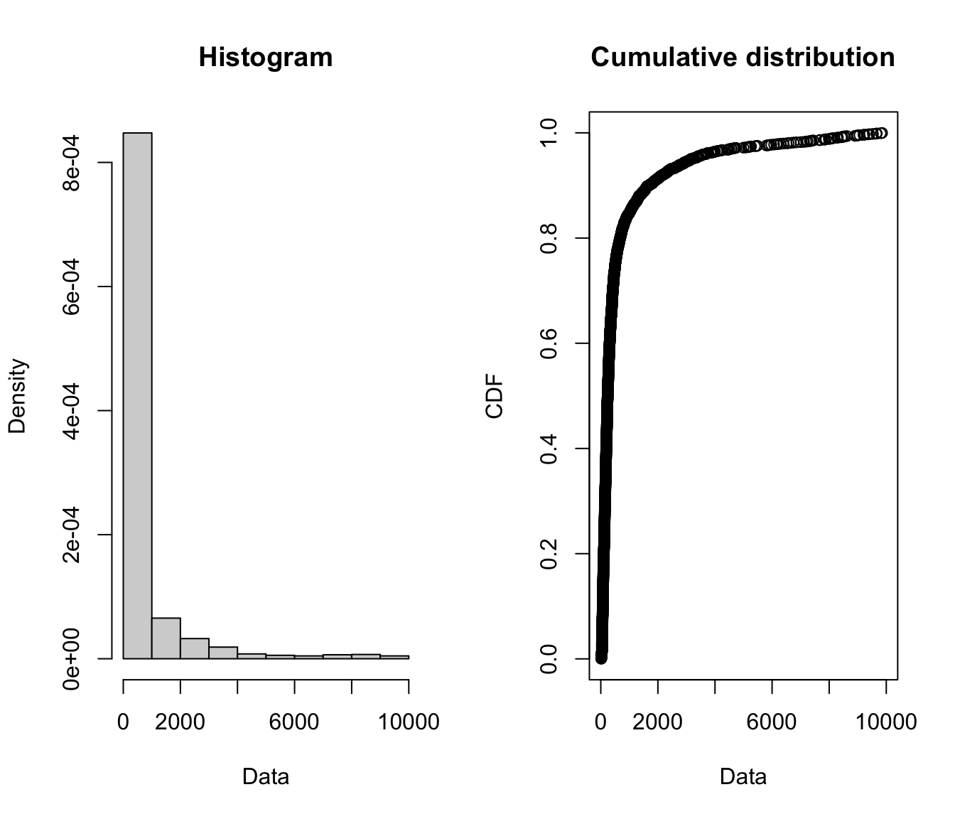
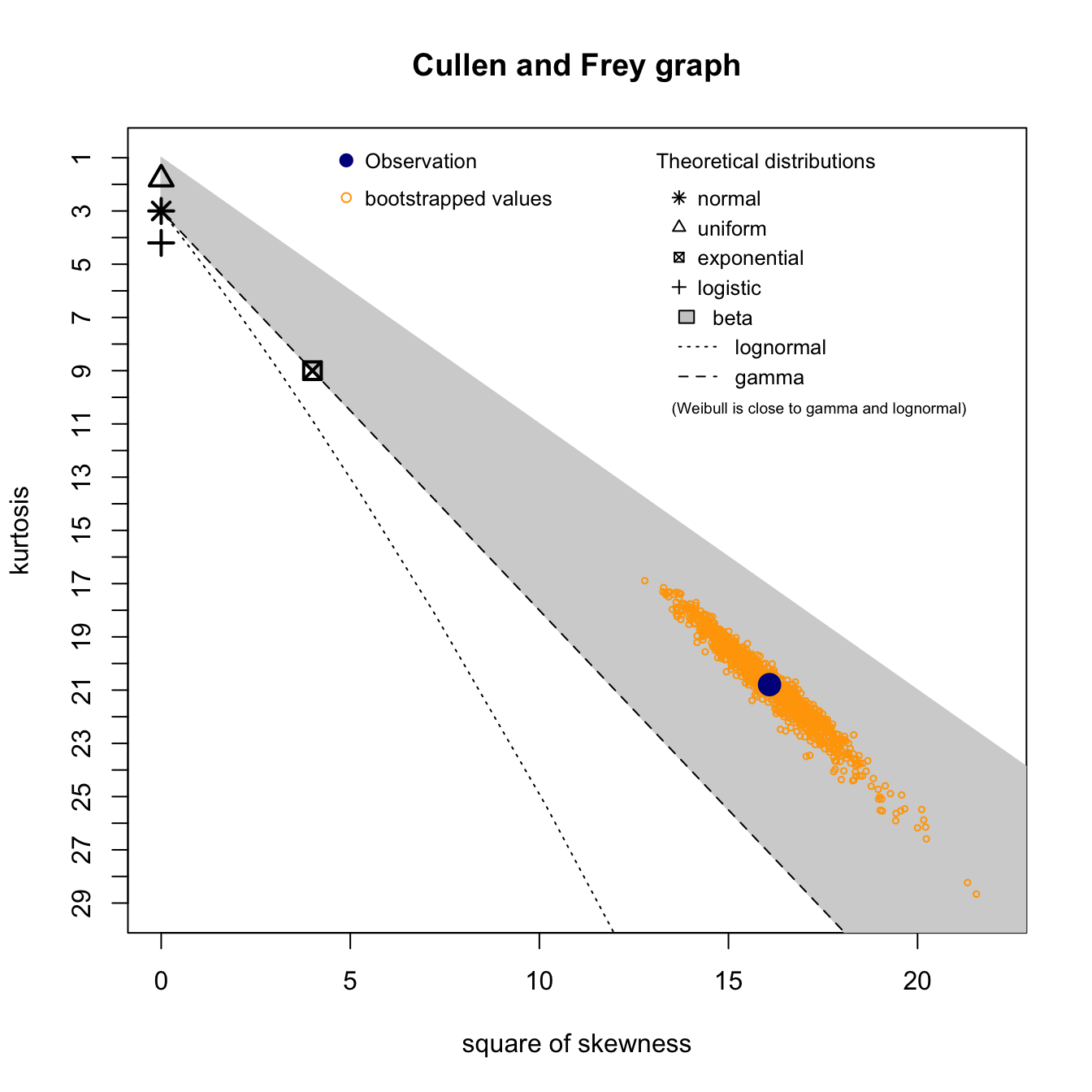
Xsc.cullen <- descdist(Xsc, boot = 1000)
Xsc.cullen
## summary statistics
## ------
## min:  15   max:  9854
## median:  240
## mean:  699.1978
## estimated sd:  1390.096
## estimated skewness:  4.010796
## estimated kurtosis:  20.79387
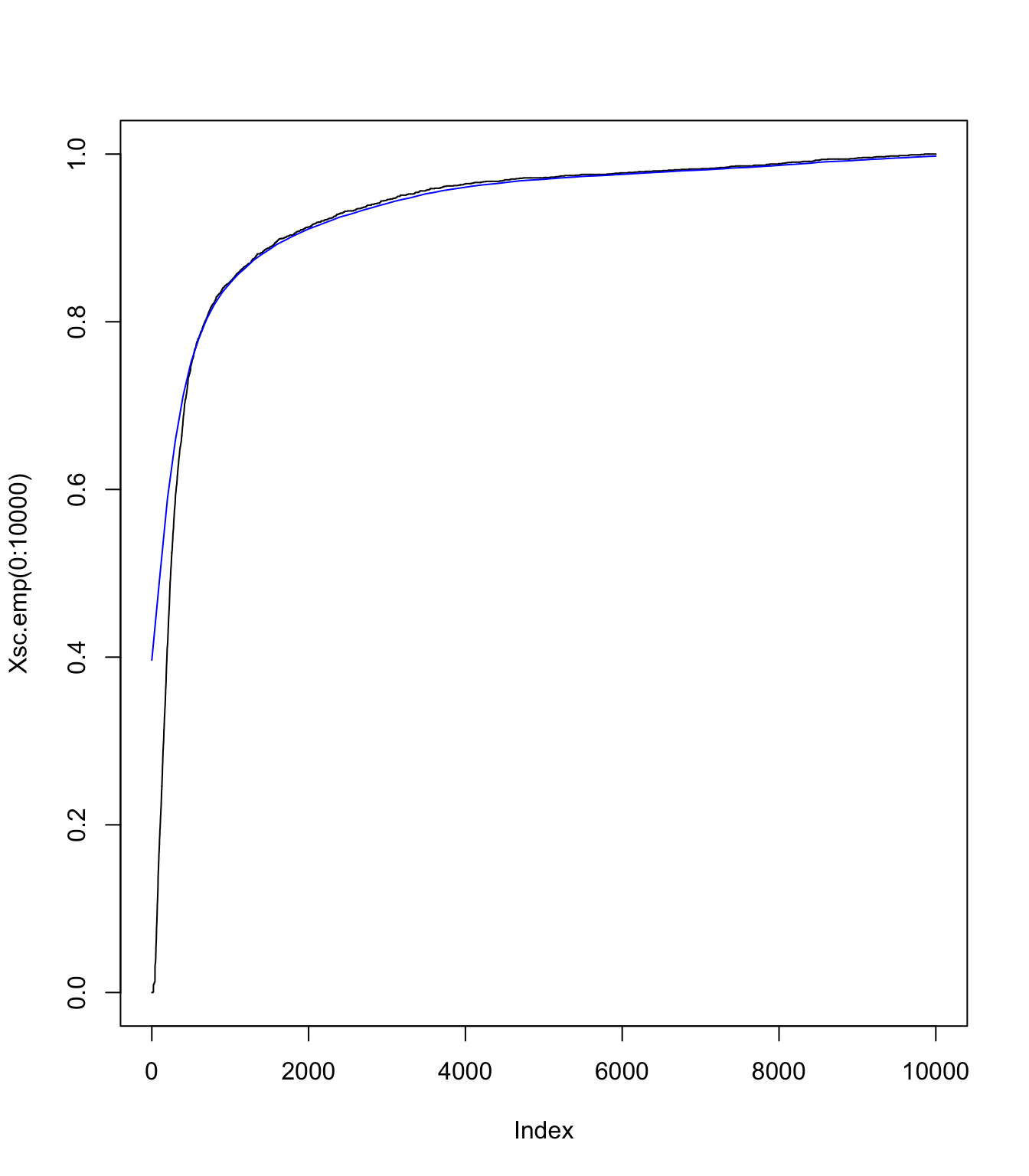
\(S_{\text{sc}}\) using the empirical distribution of \(X_{\text{sc}}\) and Panjer
#
Xsc.emp <- ecdf(Xsc)
Xsc.emp.pmf <- discretize(Xsc.emp, from = 0, to = M, step = data.scale,
  method = "rounding")
sum(Xsc.emp.pmf)
## [1] 1
# and this the cdf
Xsc.emp.df <- cumsum(Xsc.emp.pmf)
# Panjer
Ssc.emp.df <- aggregateDist(method = "recursive", model.freq = "poisson",
  model.sev = Xsc.emp.pmf, lambda = lambda.sc, x.scale = data.scale,
  maxit = 1000)
# Ssc pmf
Ssc.emp.pmf <- diff(Ssc.emp.df)
# plotting the fit
plot(Xsc.emp(0:10000), type = "l", col = "black")
lines((0:(M/data.scale) * data.scale), Ssc.emp.df((0:(M/data.scale) *
  data.scale)), pch = "-", col = "blue")
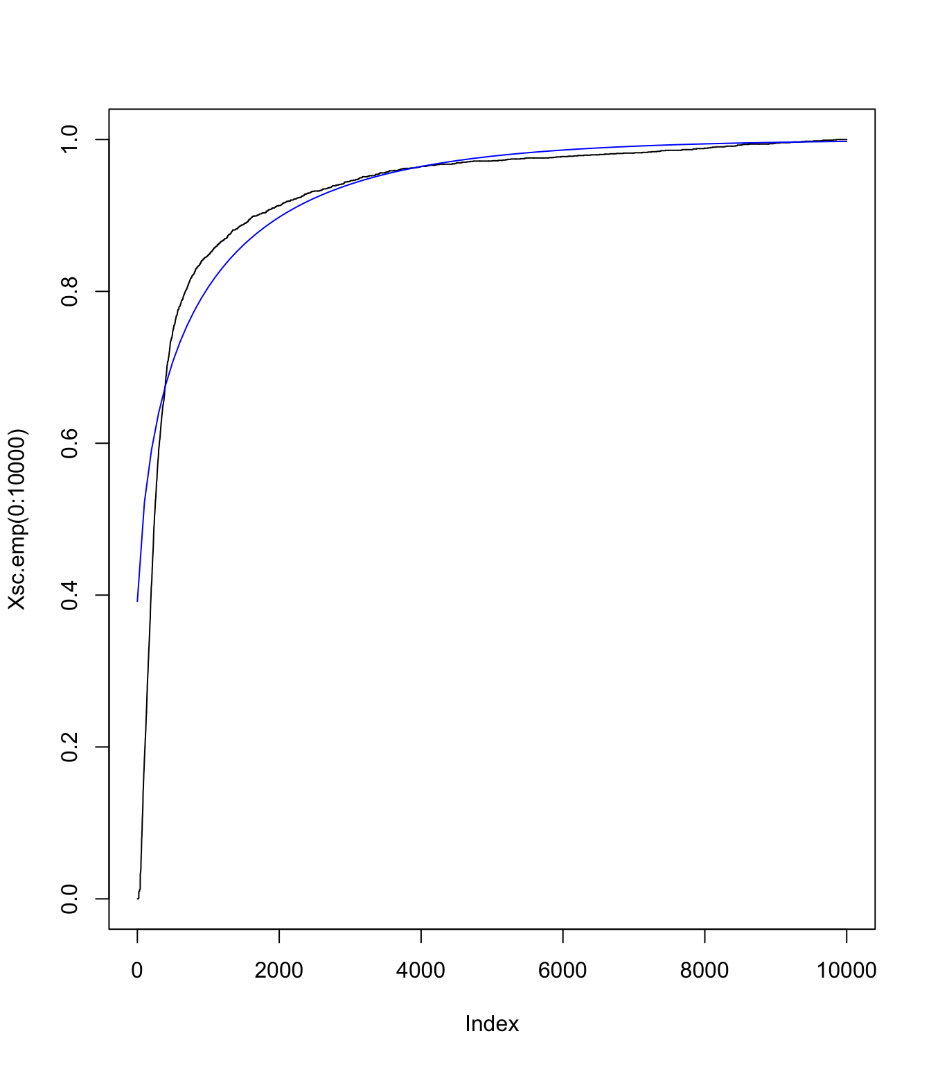
\(S_{\text{sc}}\) using an translated gamma approximation
#
# Moments of Xsc:
moments <- c(Xsc.cullen$mean, Xsc.cullen$sd^2, Xsc.cullen$skewness)
# getting parameters of translated gamma:
gamma <- (2/moments[3])^2
c <- (gamma/moments[2])^(1/2)
k <- moments[1] - gamma/c
# checking moments match:
c(gamma/c + k, moments[1])
## [1] 699.1978 699.1978
c((gamma/c^2), moments[2])
## [1] 1932366 1932366
c(2 * gamma^(-1/2), moments[3])
## [1] 4.010796 4.010796
No Panjer here - just discretisation of the gamma:
Ssc.tlg.pmf <- discretize(pgamma(x - k, shape = gamma, rate = c),
  from = 0, to = 3 * M, step = data.scale, method = "rounding")
Ssc.tlg.df <- cumsum(Ssc.tlg.pmf)
plot(Xsc.emp(0:10000), type = "l", col = "black")
lines((0:(M/data.scale) * data.scale), Ssc.tlg.df[1:(M/data.scale +
  1)], pch = "-", col = "blue")
One can see with this graph that the right tail is good (as expected), but the left tail not so much. It will be interesting to compare final results with the ecdf version (which would have a better match on this graph obviously)
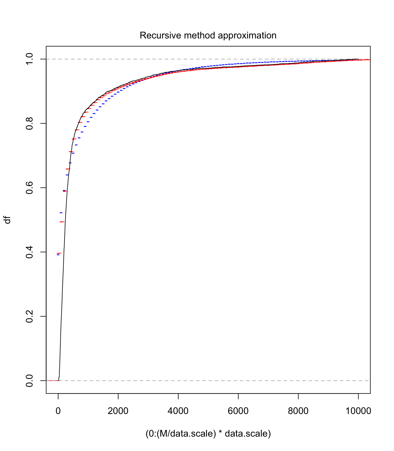
Comparison #
plot((0:(M/data.scale) * data.scale), Ssc.tlg.df[1:(M/data.scale +
  1)], pch = "-", col = "blue", xlim = c(0, 10000), ylim = c(0,
  1), ylab = "df")
lines(Ssc.emp.df, pch = "-", col = "red")
lines(Xsc.emp(0:10000), type = "l", col = "black")
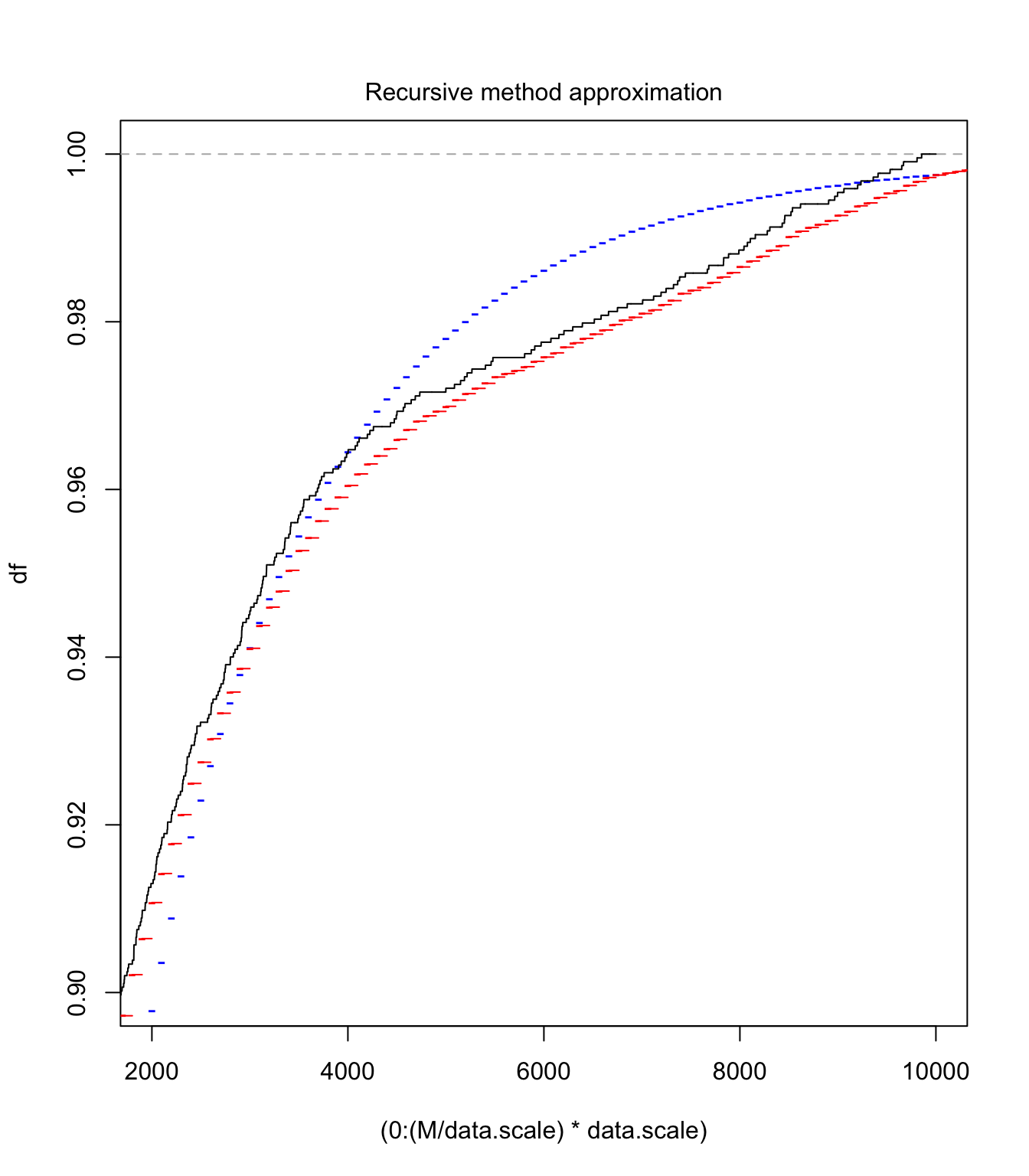
plot((0:(M/data.scale) * data.scale), Ssc.tlg.df[1:(M/data.scale +
  1)], pch = "-", col = "blue", xlim = c(2000, 10000), ylim = c(0.9,
  1), ylab = "df")
lines(Ssc.emp.df, pch = "-", col = "red")
lines(Xsc.emp(0:10000), type = "l", col = "black")
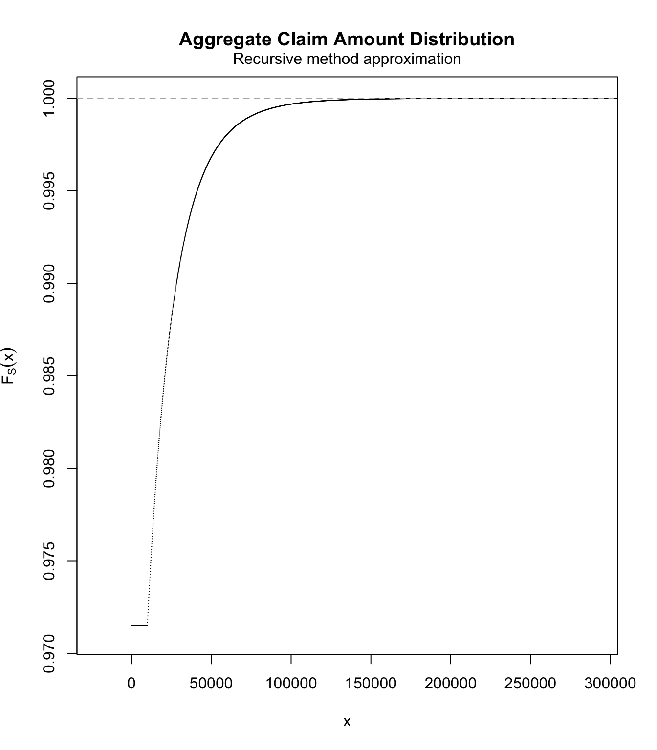
Modelling the large claims #
fit.SUVA <- fevd(SUVA$medcosts, threshold = M, type = "GP", time.units = "1/year")
# do we have mass below M?
pextRemes(fit.SUVA, M, lower.tail = TRUE)
## [1] 0
# getting the pmf:
Xlc.pmf <- discretize(pextRemes(fit.SUVA, x, lower.tail = TRUE),
  from = 0, to = 1e+06, step = data.scale)
sum(Xlc.pmf)
## [1] 1
# distribution of Slc
Slc.df <- aggregateDist(method = "recursive", model.freq = "poisson",
  model.sev = Xlc.pmf, lambda = lambda.lc, x.scale = data.scale,
  maxit = 50000)
plot(Slc.df, ylim = c(lambda.sc, 1))
# pmf of Slc
Slc.pmf <- diff(Slc.df)
Getting the overall distribution #
Getting ready #
# we'll put the masses in here
Stotal.emp.pmf <- c()
Stotal.tlg.pmf <- c()
# working out vector sizes
lastpoint <- 1e+06
masses <- lastpoint/data.scale + 1
# adding 0's as required for the convolutions to work
Ssc.emp.pmf <- c(Ssc.emp.pmf, rep(0, masses - length(Ssc.emp.pmf)))
Ssc.tlg.pmf <- c(Ssc.tlg.pmf, rep(0, masses - length(Ssc.tlg.pmf)))
Slc.pmf <- c(Slc.pmf, rep(0, masses - length(Slc.pmf)))
Performing the convolutions #
# and the convolutions
for (i in 1:masses) {
  Stotal.emp.pmf[i] <- sum(Ssc.emp.pmf[1:i] * Slc.pmf[i:1])
  Stotal.tlg.pmf[i] <- sum(Ssc.tlg.pmf[1:i] * Slc.pmf[i:1])
}
sum(Stotal.emp.pmf)
## [1] 0.999998
sum(Stotal.tlg.pmf)
## [1] 0.9999981
Stotal.emp.cdf <- cumsum(Stotal.emp.pmf)
Stotal.tlg.cdf <- cumsum(Stotal.tlg.pmf)
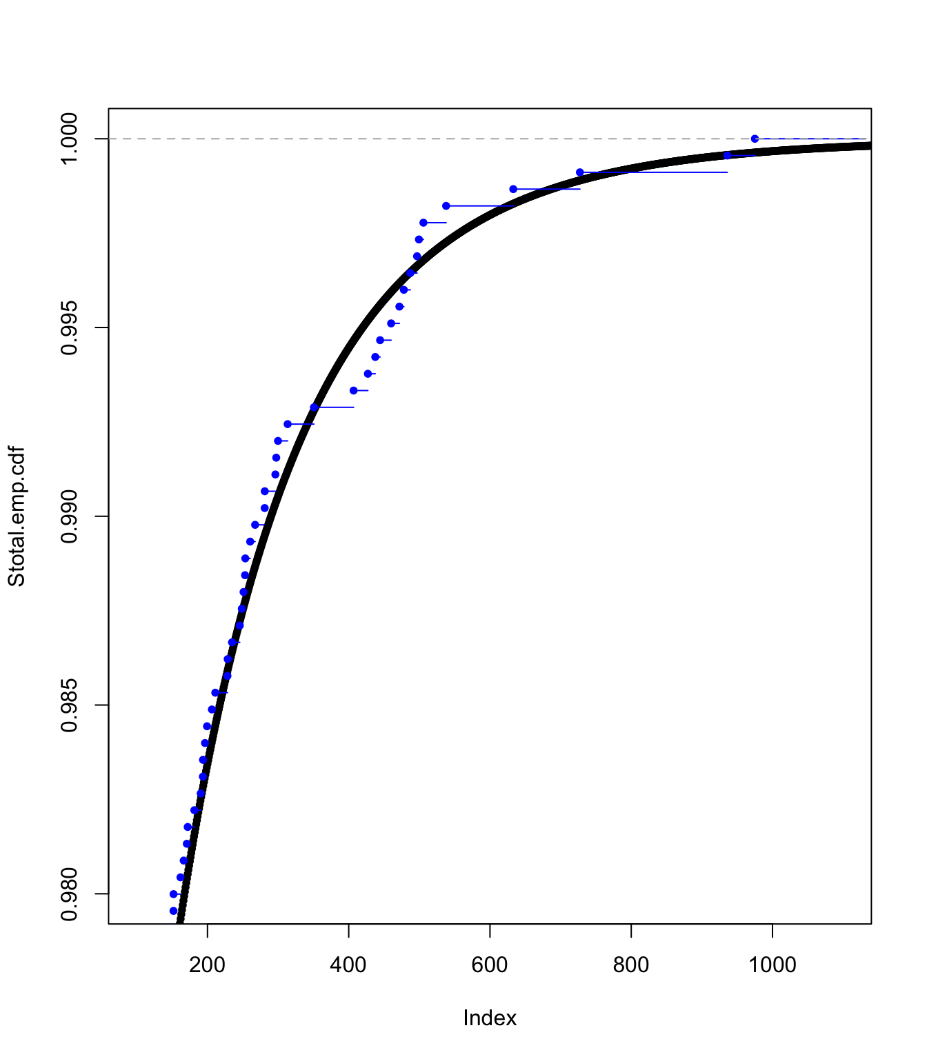
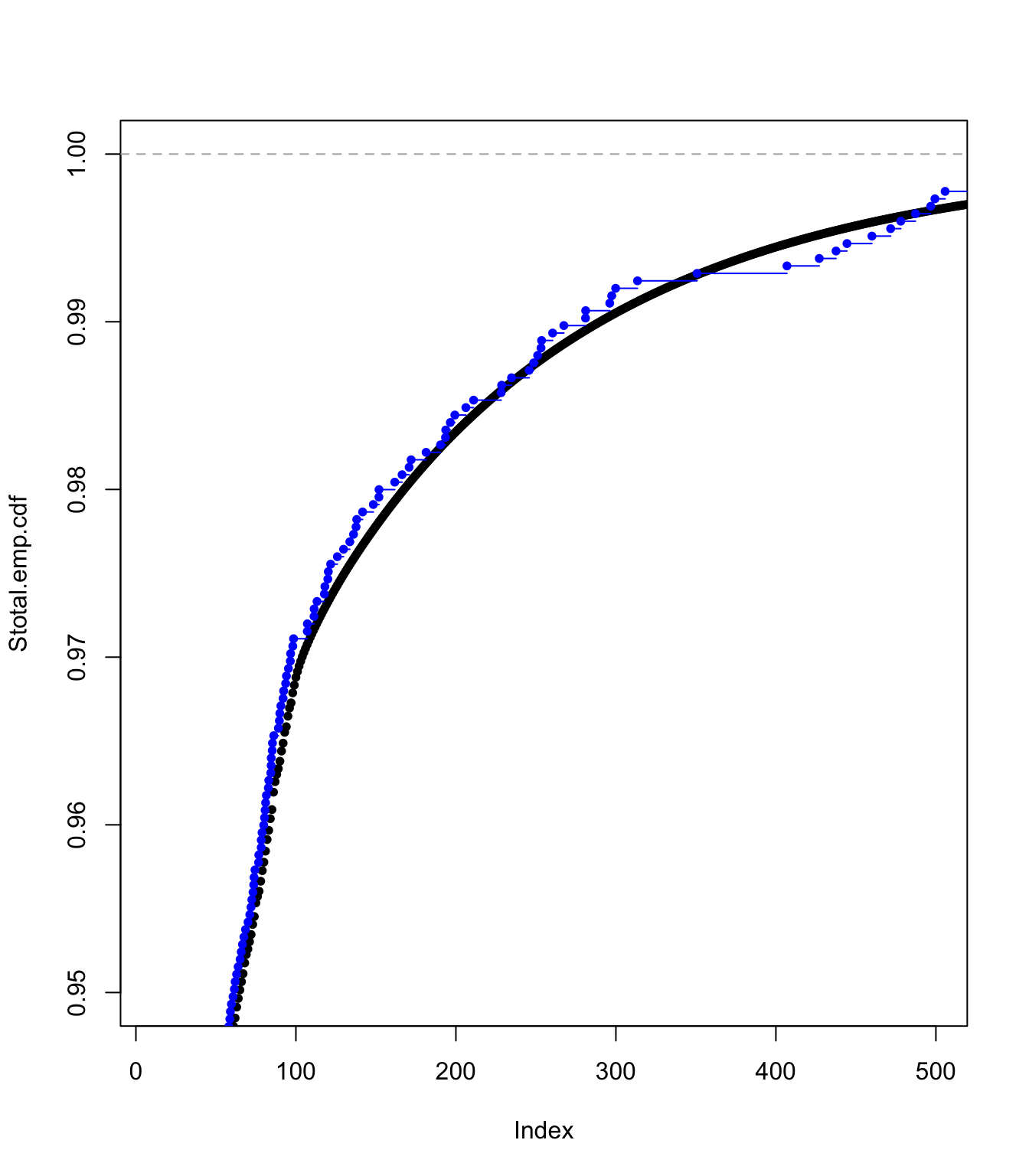
Examining the ECDF approach fit #
plot(Stotal.emp.cdf, pch = 20, xlim = c(100, 1100), ylim = c(0.98,
  1))
lines(ecdf(SUVA$medcosts[SUVA$medcosts > 0]/data.scale), pch = 20,
  col = "blue")
plot(Stotal.emp.cdf, pch = 20, xlim = c(10, 500), ylim = c(0.95,
  1))
lines(ecdf(SUVA$medcosts[SUVA$medcosts > 0]/data.scale), pch = 20,
  col = "blue")
plot(Stotal.emp.cdf, pch = 20, xlim = c(0, 500), ylim = c(0.9,
  1))
lines(ecdf(SUVA$medcosts[SUVA$medcosts > 0]/data.scale), pch = 20,
  col = "blue")
plot(Stotal.emp.cdf, pch = 20, xlim = c(0, 20), ylim = c(0, 1))
lines(ecdf(SUVA$medcosts[SUVA$medcosts > 0]/data.scale), pch = 20,
  col = "blue")


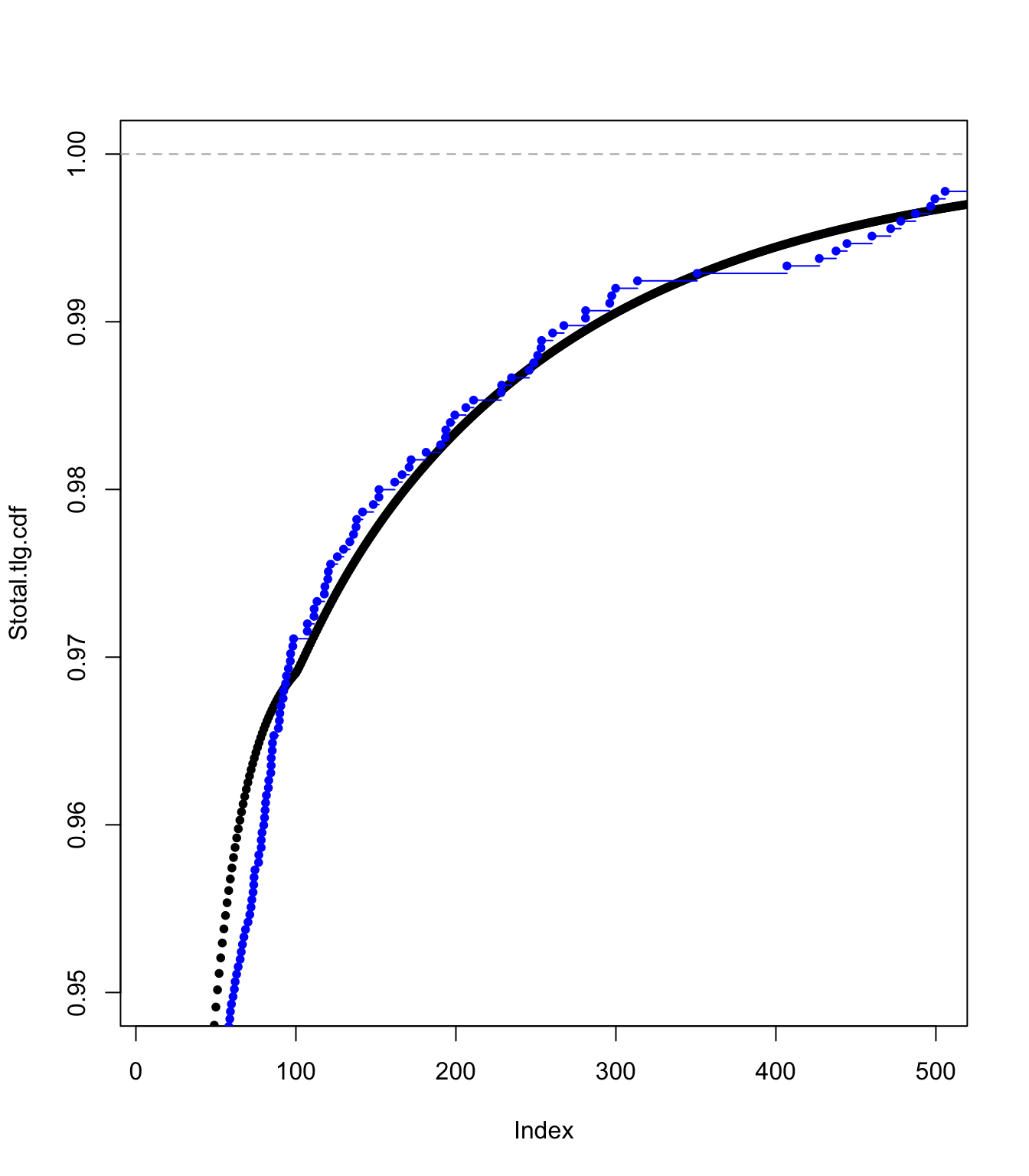
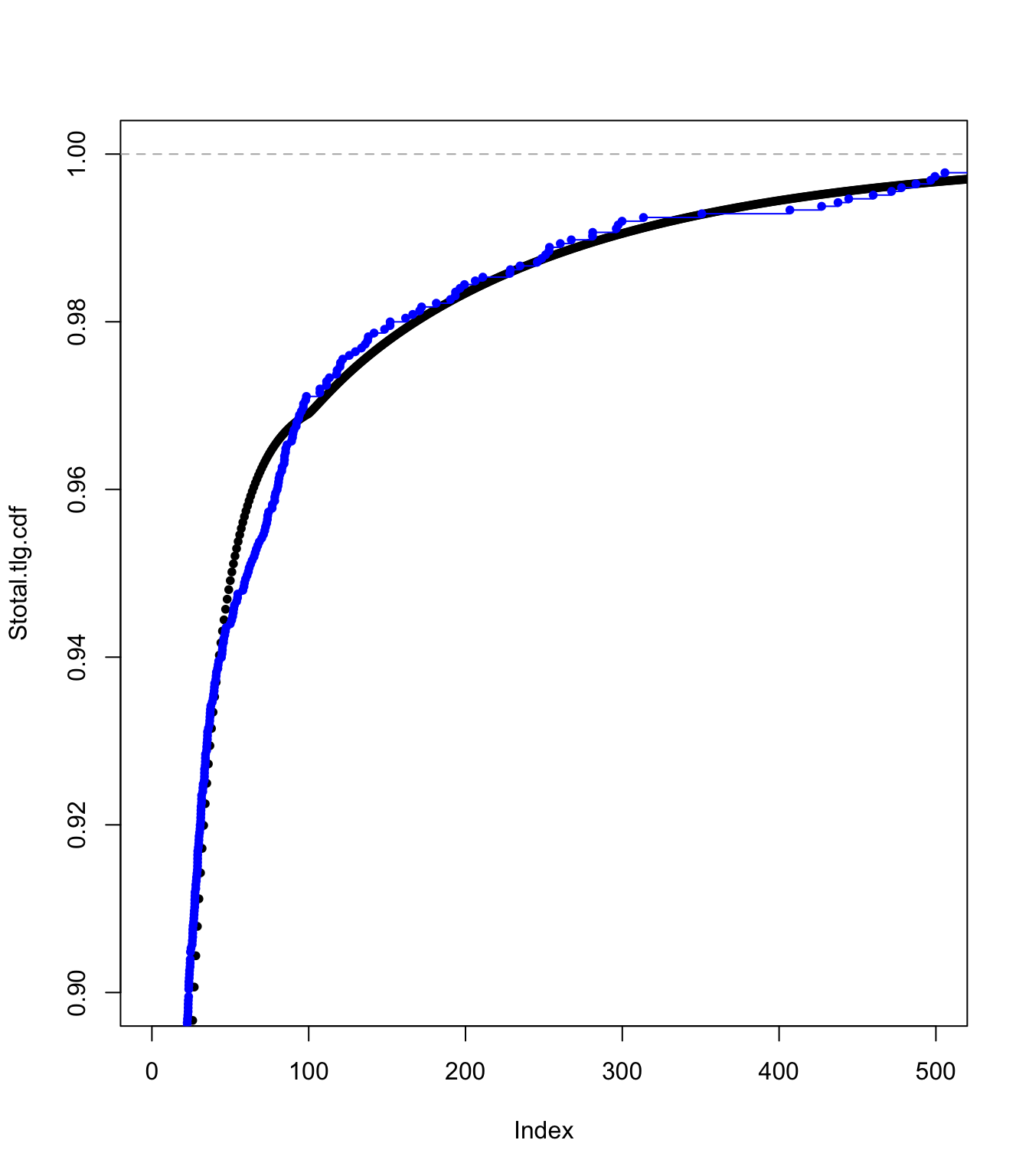
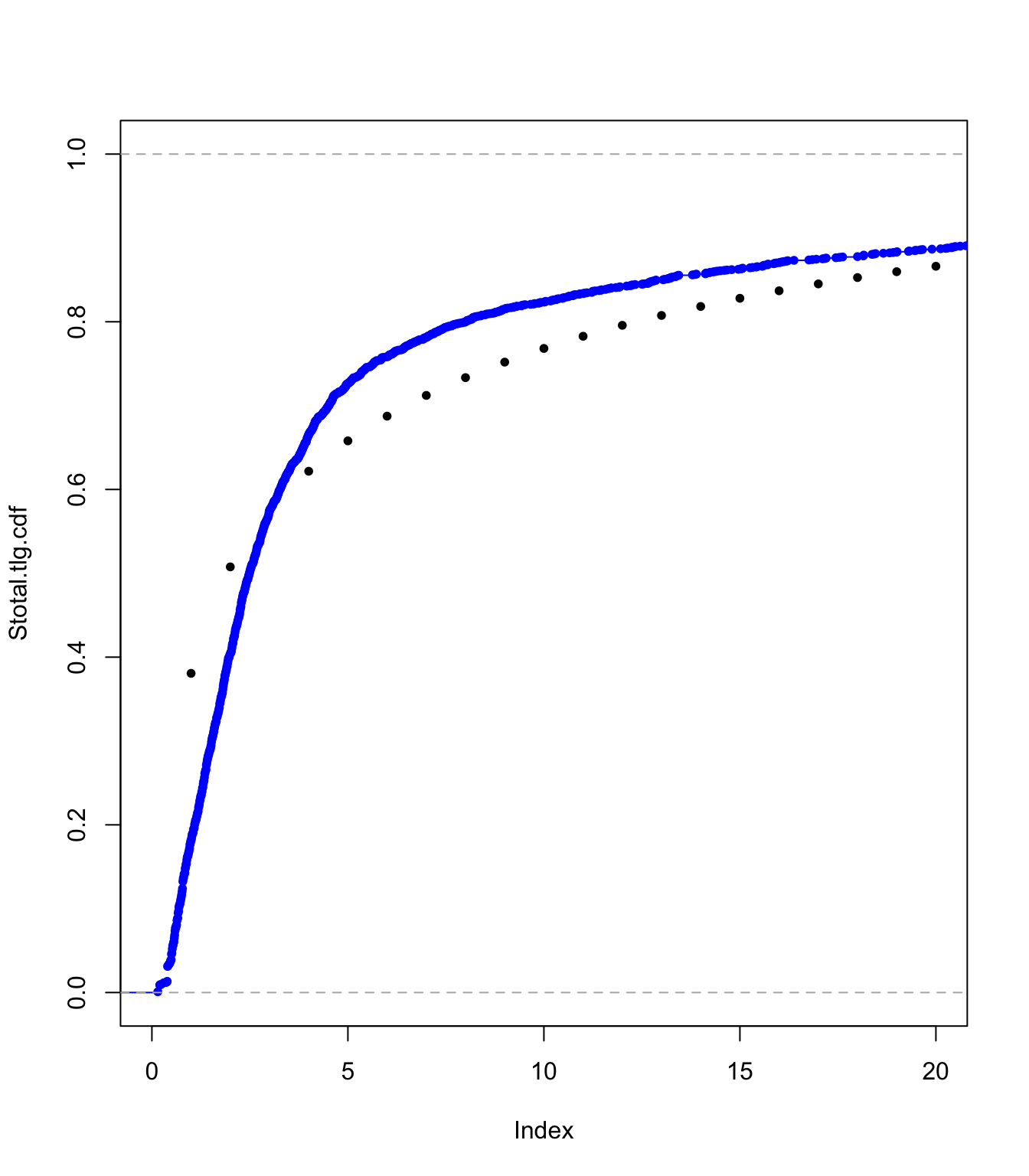
Examining the translated gamma approach fit #
plot(Stotal.tlg.cdf, pch = 20, xlim = c(100, 1100), ylim = c(0.98,
  1))
lines(ecdf(SUVA$medcosts[SUVA$medcosts > 0]/data.scale), pch = 20,
  col = "blue")
plot(Stotal.tlg.cdf, pch = 20, xlim = c(10, 500), ylim = c(0.95,
  1))
lines(ecdf(SUVA$medcosts[SUVA$medcosts > 0]/data.scale), pch = 20,
  col = "blue")
plot(Stotal.tlg.cdf, pch = 20, xlim = c(0, 500), ylim = c(0.9,
  1))
lines(ecdf(SUVA$medcosts[SUVA$medcosts > 0]/data.scale), pch = 20,
  col = "blue")
plot(Stotal.tlg.cdf, pch = 20, xlim = c(0, 20), ylim = c(0, 1))
lines(ecdf(SUVA$medcosts[SUVA$medcosts > 0]/data.scale), pch = 20,
  col = "blue")

Moments #
em1 <- c(emm(SUVA$medcosts[SUVA$medcosts > 0], 1), sum((((1:masses) -
  1) * data.scale) * (Stotal.emp.pmf)), sum((((1:masses) -
  1) * data.scale) * (Stotal.tlg.pmf)))
em2 <- c(emm(SUVA$medcosts[SUVA$medcosts > 0], 2), sum((((1:masses) -
  1) * data.scale)^2 * (Stotal.emp.pmf)), sum((((1:masses) -
  1) * data.scale)^2 * (Stotal.tlg.pmf)))
em3 <- c(emm(SUVA$medcosts[SUVA$medcosts > 0], 3), sum((((1:masses) -
  1) * data.scale)^3 * (Stotal.emp.pmf)), sum((((1:masses) -
  1) * data.scale)^3 * (Stotal.tlg.pmf)))
sd <- (em2 - em1^2)^0.5
skew <- (em3 - 3 * em1 * sd^2 - em1^3)/sd^3
Smoments <- data.frame(rbind(em1, sd, skew))
names(Smoments) <- c("SUVA", "Emp", "Tlg")
Smoments
##             SUVA         Emp         Tlg
## em1  1492.765229 1478.788445 1494.851875
## sd   5763.108871 5932.145105 5897.220298
## skew    8.885693    9.739098    9.893872
References #
Avanzi, Benjamin, Luke C. Cassar, and Bernard Wong. 2011. “Modelling Dependence in Insurance Claims Processes with Lévy Copulas.” ASTIN Bulletin 41 (2): 575–609.
Bowers, Newton L. Jr, Hans U. Gerber, James C. Hickman, Donald A. Jones, and Cecil J. Nesbitt. 1997. Actuarial Mathematics. Second. Schaumburg, Illinois: The Society of Actuaries.
Wuthrich, Mario V. 2023. “Non-Life Insurance: Mathematics & Statistics.” Lecture notes. RiskLab, ETH Zurich; Swiss Finance Institute.