Introduction #
- How to fit loss models to insurance data?
- Peculiar characteristics of insurance data:
- complete vs incomplete set of observations
- left-truncated observations
- right-censored observations
- heavy tailed risks
- Parametric distribution models
- model parameter estimation
- judging quality of fit
- model selection criteria
(graphical, score-based approaches, information criteria)
- Concepts and R functions are demonstrated with the help of some data sets
Steps in fitting loss models to data #
- explore and summarise data
- graphical explorations
- empirical moments and quantiles
- select a set of candidate distributions
- Pareto, log-normal, inverse Gaussian, gamma, etc.
- estimate the model parameters
- method of moments
- maximum likelihood (MLE)
- maximum goodness (MGE)
- evaluate the quality of a given model
- graphical procedures (qq, pp plots, empirical cdf’s)
- score-based approaches (Kolmogorov-Smirnoff tests, AD tests, chi-square goodness-of-fit tests)
- likelihood based information criteria (AIC, BIC)
- determine which model to choose based on needs
Insurance data #
Complete vs incomplete data #
- complete, individual data
- you observe the exact value of the loss
- incomplete data
- exact data may not be available
- in loss/claims data, these arise in the following situations:
- observations may be grouped - observe only the range of values in which the data belongs
- presence of censoring and/or truncation
- due to typical insurance and reinsurance arrangements such as deductibles and limits
Left-truncation and right-censoring #
- left-truncated observation (e.g. excess / deductible)
- observation is left-truncated at
\(c\)if it is NOT recorded when it is below\(c\)and when it is above\(c\), it is recorded at its exact value.
- observation is left-truncated at
- right-censored observation (e.g. policy limit)
- observation is right-censored at
\(d\)if when it is above\(d\)it is recorded as being equal to\(d\)but when it is below\(d\)it is recorded at its observed value.
- observation is right-censored at
- similarly, we can define right-truncated, left-censored,
\(\ldots\) - of course, observations can be both left-truncated and right-censored; this is often the case in actuarial data
Zero claims #
- Significant proportions of zero claims are frequent, for a number of reasons:
- Data is policy-based, not claims-based;
- Claim not exceeding deductible;
- Mandatory reporting of accidents;
- etc…
- This complicates the fitting (parametric distributions often don’t have a flexible mass at 0, if at all)
- Several possible solutions
- Adjust
\(Y\)by mixing 0 with a parametric distribution - Adjust the frequency of claims accordingly (hence ignoring 0 claims), but this
- may understate the volatility of claims (the proportion of 0’s may also be random)
- should be avoided if 0’s are claims of no cost (rather than absence of claim)
- Adjust
Heavy tailed risks #
- Essentially, these are risks that can be very large.
- This is translated by thick tails, that is, a density that goes to zero slowly in the tails.
- Typically, this means that the expectation of the excess over a threshold increases with that threshold.
- We will encounter such losses here, but a full treatment is deferred to Module 6 (Extreme Value Theory).
Data set used for illustrations #
Bivariate data set of Swiss workers compensation medical and daily allowance costs:
- Example of real actuarial data; see Avanzi, Cassar, and Wong (2011)
- Data were provided by the SUVA (Swiss workers compensation insurer)
- Random sample of 5% of accident claims in construction sector with accident year 1999 (developped as of 2003)
- Claims are (joint) medical costs and daily allowance costs
SUVA <- read_excel("SUVA.xls")
as_tibble(SUVA)
...
## # A tibble: 2,326 × 2
##    medcosts dailyallow
##       <dbl>      <dbl>
##  1      407          0
##  2    12591      13742
##  3      269          0
##  4      142          0
##  5      175          0
##  6      298        839
##  7       47          0
...
Data analysis and descriptive statistics (MW 3.1) #
It is essential, before any modelling is done, to make sure that one gets a good sense of what the data look like.
- For any type of data analysis, first thing to do is to summarise the data.
- summary statistics: mean, median, standard deviation, coefficient of variation, skewness, quantiles, min, max, etc
\(\ldots\) - gives a preliminary understanding of the data
- summary statistics: mean, median, standard deviation, coefficient of variation, skewness, quantiles, min, max, etc
- Visualisating the data is often even more informative:
- histogram, with associated kernel density
- empirical cdf, which can be compared to that of a normal cdf via Q-Q or P-P plot
- When data are heavy tailed it often helps to perform the above on the log of the data (we can then compare the data to a lognormal)
- Data collection procedures and standards should be understood
- Any unusual feature (outliers, breaks, …) should be investigated. If possible, ask the claims adjusters or data owners about them
Raw data #
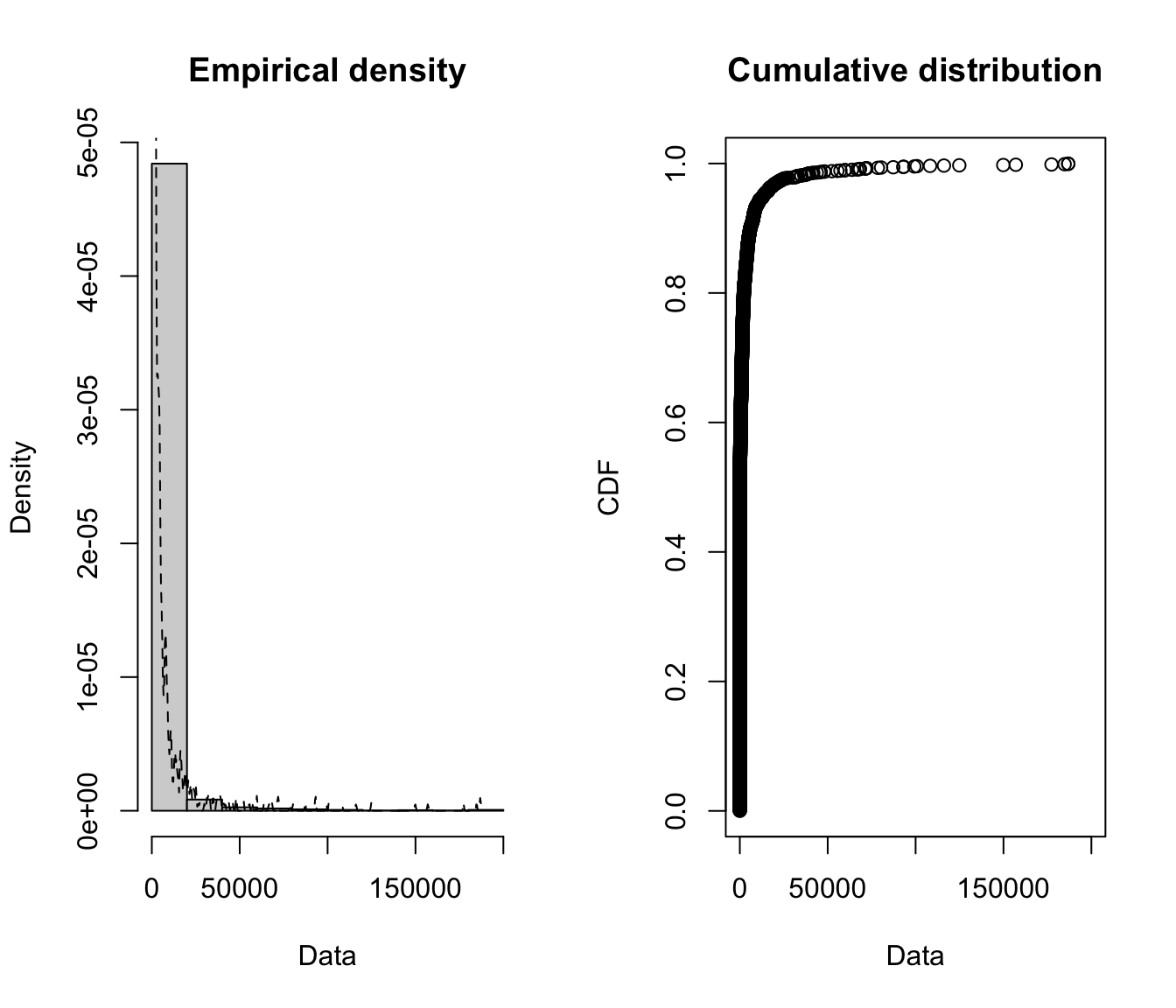
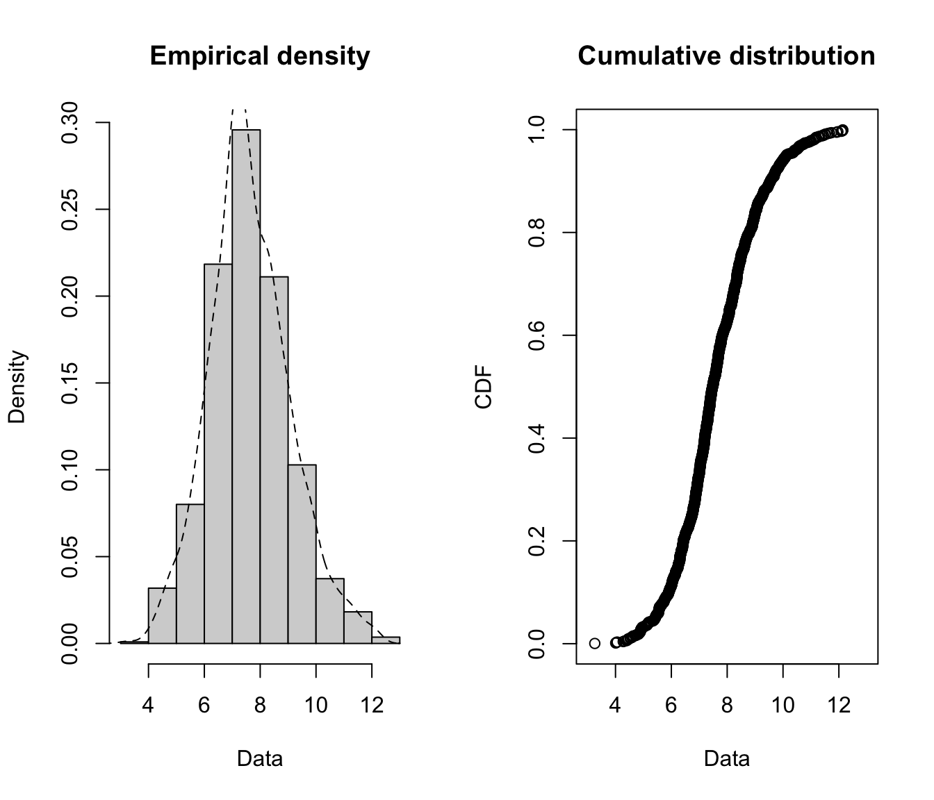
Visualise the SUVA raw data #
fitdistrplus::plotdist(SUVA$medcosts, histo = TRUE, demp = TRUE)
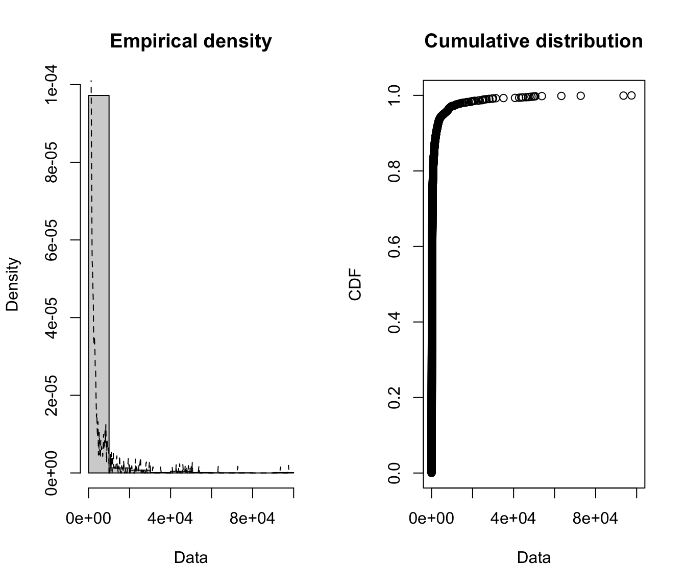
plotdist(SUVA$dailyallow, histo = TRUE, demp = TRUE)
plotdist(SUVA$dailyallow[SUVA$dailyallow > 0], histo = TRUE,
  demp = TRUE)
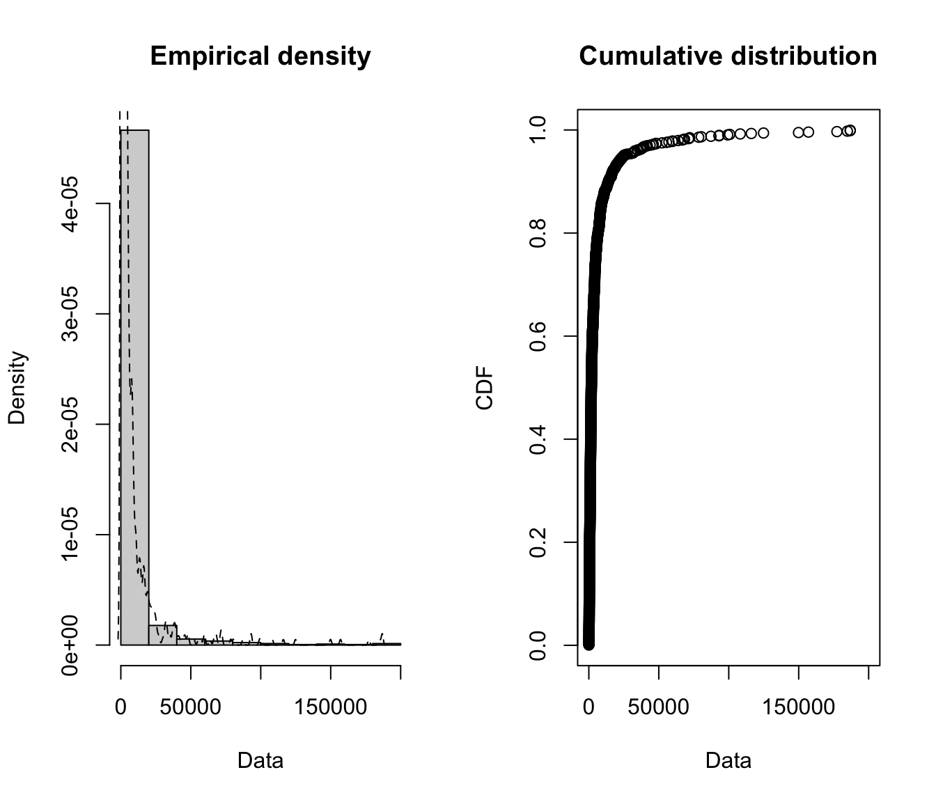
A log transformation may help us see better what is happening.
log of raw SUVA data #
plotdist(log(SUVA$medcosts[SUVA$medcosts > 0]), histo = TRUE,
  demp = TRUE)
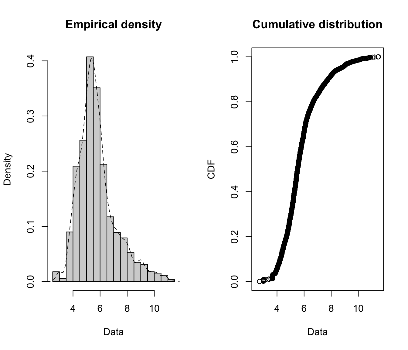
plotdist(log(SUVA$dailyallow[SUVA$dailyallow > 0]), histo = TRUE,
  demp = TRUE)
- Medical costs are still skewed even after a log transformation, which suggests that a very heavy tailed distribution might be necessary.
- Daily allowance costs look symmetrical after the log transformation, which suggests a lognormal (or similar) distribution might be appropriate.
- Removing 0’s is especially important for the daily allowance claims (and is necessary for taking the log anyway), as more than half of the claims are 0.
Moments #
Moments of a distribution provide information:
- The mean provides its location
- The second moment leads to the variance, and the coefficient of variation, which give an idea of the dispersion around the mean
- Skewness is self-explanatory
- Kurtosis provides an idea of how fat the tails are
- “Excess Kurtosis” is with respect to a normal/logonormal distribution for raw/log claims, respectively
The following are also helpful:
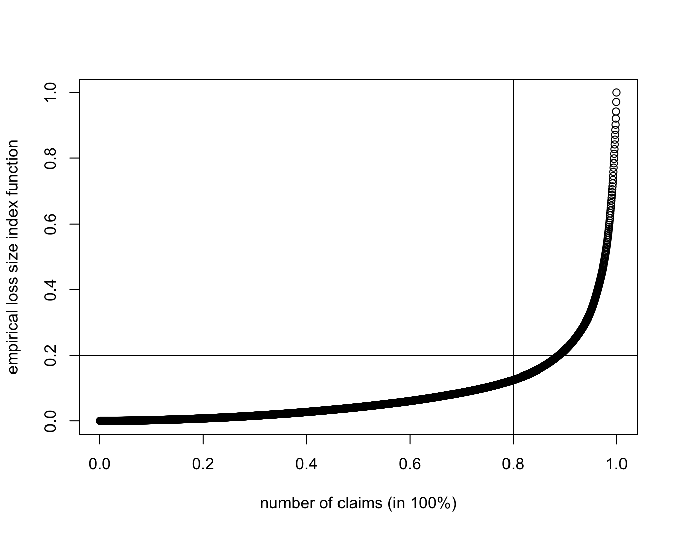
- Loss size index function
$$\mathcal{I}(G(y)) = \frac{\int_0^y z dG(z)}{\int_0^\infty z dG(z)} \quad \text{and} \quad \widehat{\mathcal{I}}_n(\alpha)=\frac{\sum_{i=1}^{\lfloor n \alpha \rfloor} Y_{(i)}}{\sum_{i=1}^n Y_i}$$for\(\alpha \in [0,1]\). Corresponds of the contribution of\([0,y]\)to the overall mean. (see also , whereby 80% of overall cost would be due to 20% of (the most costly) claims) - Mean excess function
$$e(u)=E[Y_i-u|Y_i>u] \quad \text{and} \quad \widehat{e}_n(u) = \frac{\sum_{i=1}^n (Y_i-u) 1_{\{Y_i>u\}}}{\sum_{i=1}^n 1_{\{Y_i>u\}}}$$This is useful for the analysis of large claims, and for the analysis of reinsurance. Increasing values of the mean excess function indicate a heavy tailed distribution (see also Module 6) [Note\(u=0\)leads to the mean only when all claims are strictly positive.]
In R:
- To get numbers:
- the function
actuar::emmprovides empirical moments up to any order mean,stats::varandstats::sdprovide mean, variance, and standard deviation (unbiased versions)- codes for the Loss size index function are provided in the illustration
- codes for the Mean excess function are also provided, but the graph is most easily plotted with
extRemes::mrlplotas will be demonstrated
- the function
- The function
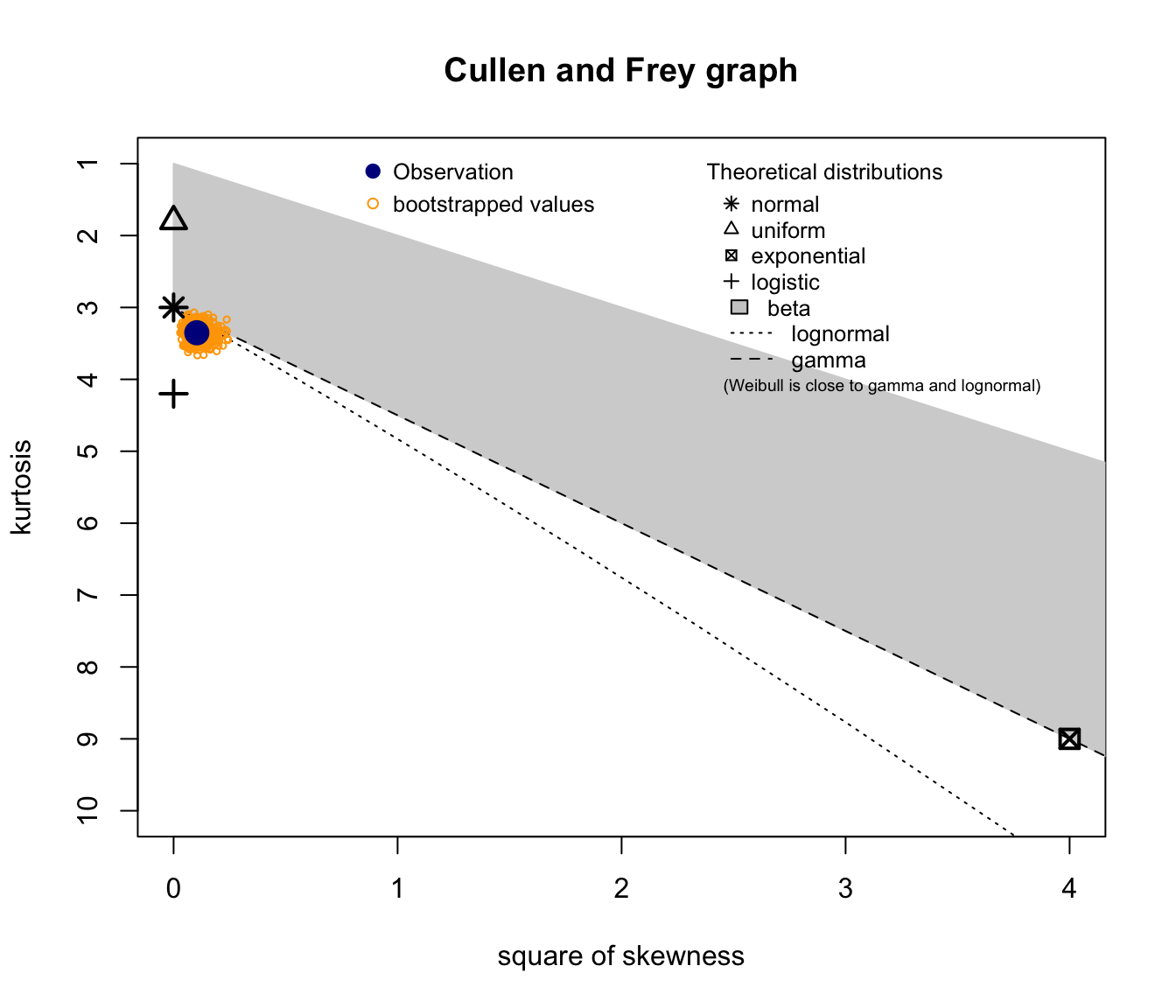
fistdistrplus:descdistprovides a graph that shows where the couple “skewness/kurtosis” lies, in comparison with its theoretically possible locations for a certain number of distributions.- the parameter
bootallows for nonparametric bootstrapping of that coordinate, which helps with the assessment of its potential variability (it is sensitive to outliers, that is, not “robust”) methodcan be"unbiased"or"sample"for the unbiased or sample versions of the moments
- the parameter
SUVA moments #
Medical costs:
format(actuar::emm(SUVA$medcosts, order = 1:3), scientific = FALSE)
## [1] " 1443.349" " 34268506.007" "1791560934502.502"
sd(SUVA$medcosts)/mean(SUVA$medcosts)
## [1] 3.93143
Daily allowance:
format(actuar::emm(SUVA$dailyallow, order = 1:3), scientific = FALSE)
## [1] " 3194.15" " 172677852.63" "20364647975482.07"
sd(SUVA$dailyallow)/mean(SUVA$dailyallow)
## [1] 3.991459
Medical costs:
format(actuar::emm(SUVA$medcosts[SUVA$medcosts > 0], order = 1:3),
  scientific = FALSE)
## [1] " 1492.765" " 35441771.887" "1852899392464.571"
sd(SUVA$medcosts[SUVA$medcosts > 0])/mean(SUVA$medcosts[SUVA$medcosts >
  0])
## [1] 3.861552
Daily allowance:
format(actuar::emm(SUVA$dailyallow[SUVA$dailyallow > 0], order = 1:3),
  scientific = FALSE)
## [1] " 6760.322" " 365467411.472" "43101156679682.695"
sd(SUVA$dailyallow[SUVA$dailyallow > 0])/mean(SUVA$dailyallow[SUVA$dailyallow >
  0])
## [1] 2.646343
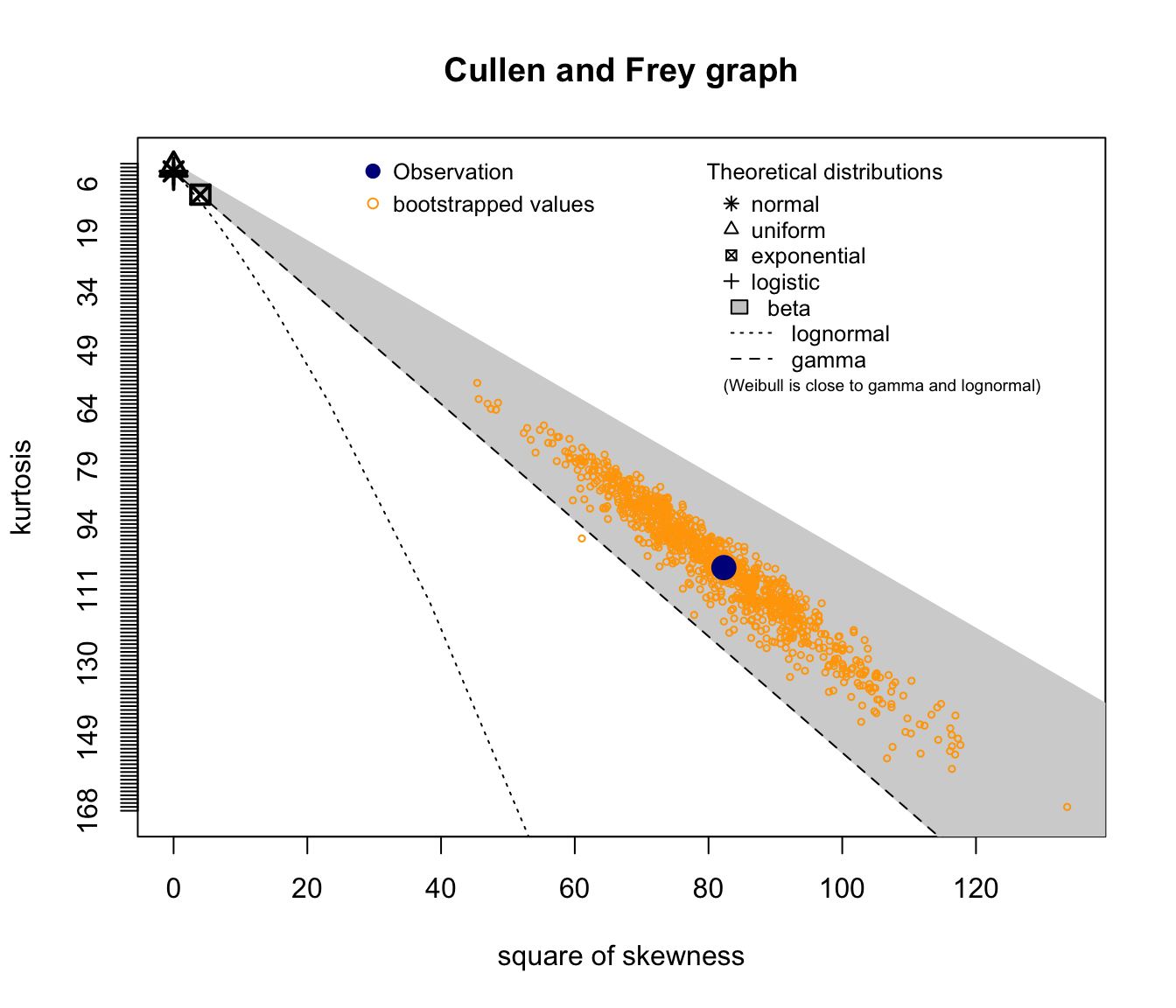
SUVA Medical Costs skewness and kurtosis #
fitdistrplus::descdist(SUVA$medcosts, boot = 1000)
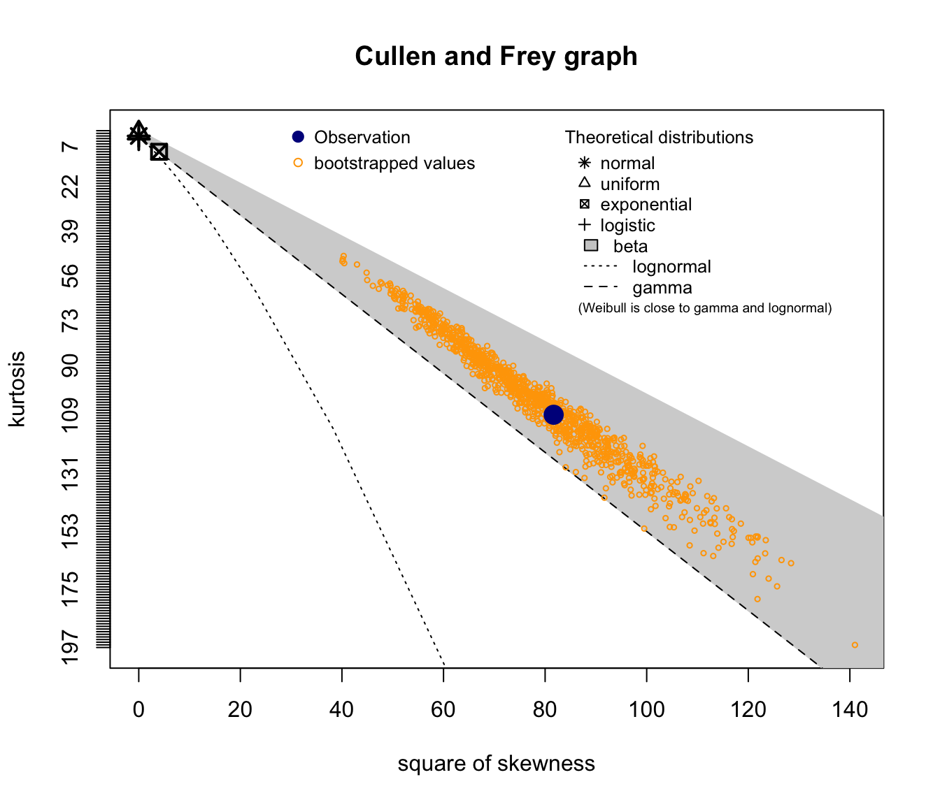
descdist(SUVA$medcosts[SUVA$medcosts > 0], boot = 1000)
descdist(log(SUVA$medcosts[SUVA$medcosts > 0]), boot = 1000)
descdist(log(log(SUVA$medcosts[SUVA$medcosts > 0])), boot = 1000)
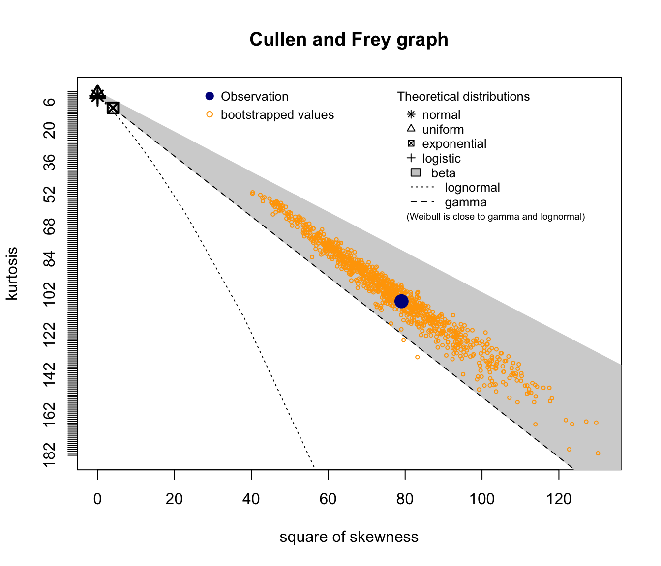
SUVA Daily Allowance skewness and kurtosis #
descdist(SUVA$dailyallow, boot = 1000)
descdist(SUVA$dailyallow[SUVA$dailyallow > 0], boot = 1000)
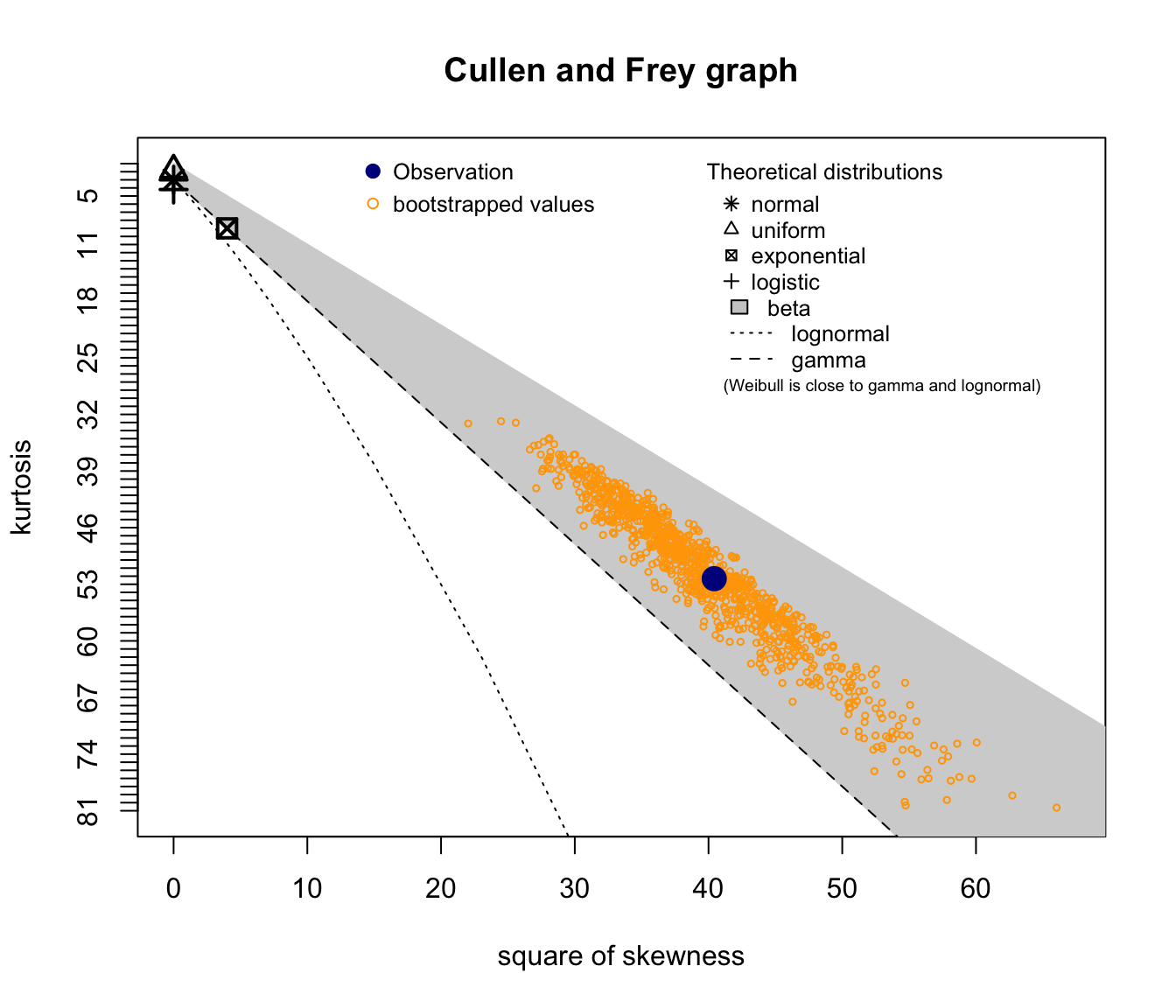
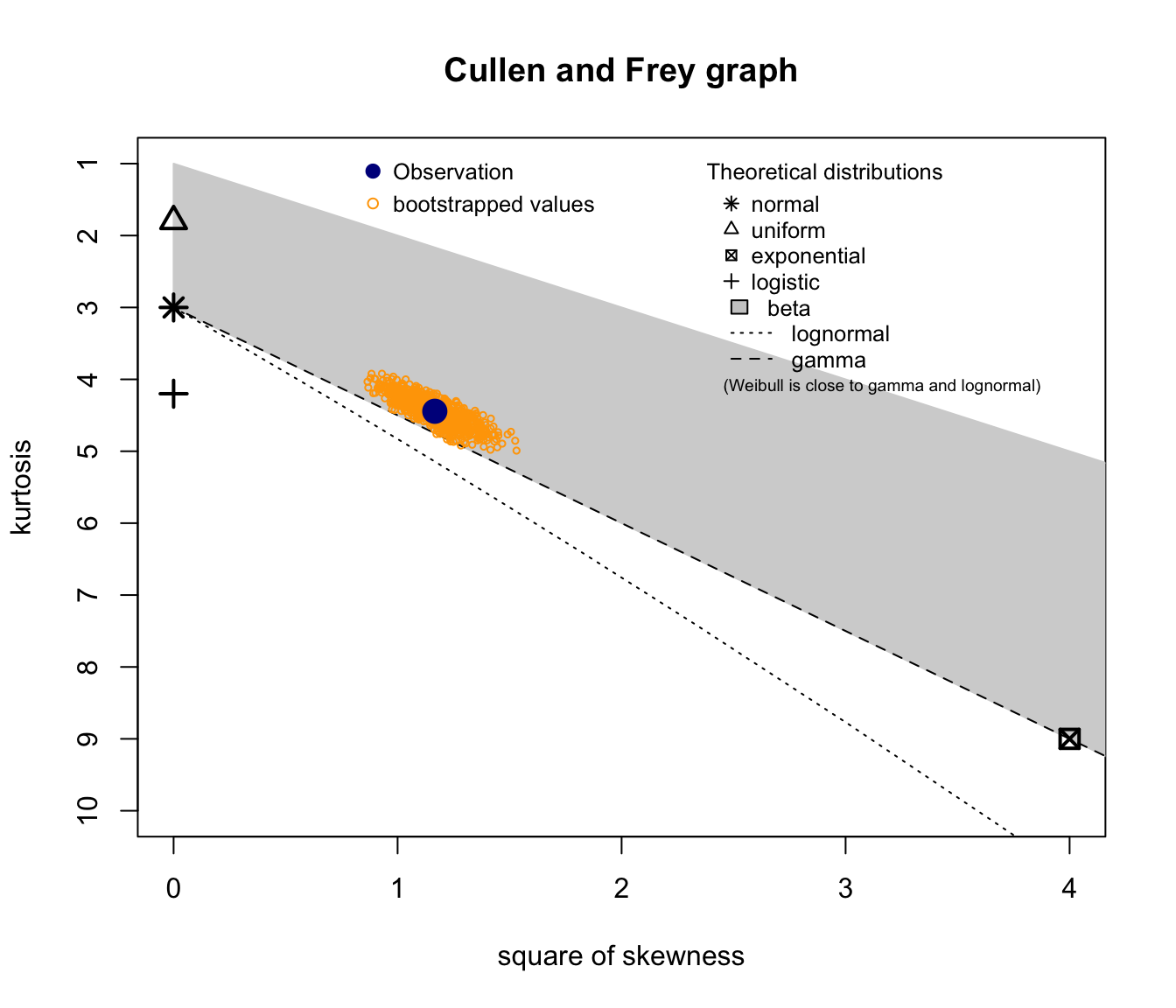
descdist(log(SUVA$dailyallow[SUVA$dailyallow > 0]), boot = 1000)
## summary statistics
## ------
## min:  3.258097   max:  12.13806
## median:  7.474772
## mean:  7.63051
## estimated sd:  1.441014
## estimated skewness:  0.3378648
## estimated kurtosis:  3.259708
Note descdist also gives stats as above!
(not shown on the previous slides)

Good candidates seem to be lognormal, gamma, and potentially Weibull.
Loss index function #
SUVA.MC.lif <- cumsum(sort(SUVA$medcosts))/sum(SUVA$medcosts)
plot(1:length(SUVA$medcosts)/length(SUVA$medcosts), SUVA.MC.lif,
  xlab = "number of claims (in 100%)", ylab = "empirical loss size index function")
abline(h = 0.2, v = 0.8)
SUVA.DA.lif <- cumsum(sort(SUVA$dailyallow))/sum(SUVA$dailyallow)
plot(1:length(SUVA$dailyallow)/length(SUVA$dailyallow), SUVA.DA.lif,
  xlab = "number of claims (in 100%)", ylab = "empirical loss size index function")
abline(h = 0.2, v = 0.8)

Mean excess function #
This function will return the mean excess function for an arbitrary vector of thresholds u (for instance, 0, 100, 1000 and 10000 here)
mef <- function(x, u) {
  mefvector <- c()
  for (i in u) {
    mefvector <- c(mefvector, sum(pmax(sort(x) - i, 0))/length(x[x >
      i]))
  }
  return(mefvector)
}
mef(SUVA$medcosts, c(0, 100, 1000, 10000))
## [1]  1492.765  1709.148  6233.296 18156.631
mean(SUVA$medcosts)
## [1] 1443.349
mean(SUVA$medcosts[SUVA$medcosts > 0])
## [1] 1492.765
The graph is best done with extRemes::mrlplot
mrlplot(SUVA$medcosts[SUVA$medcosts > 0])
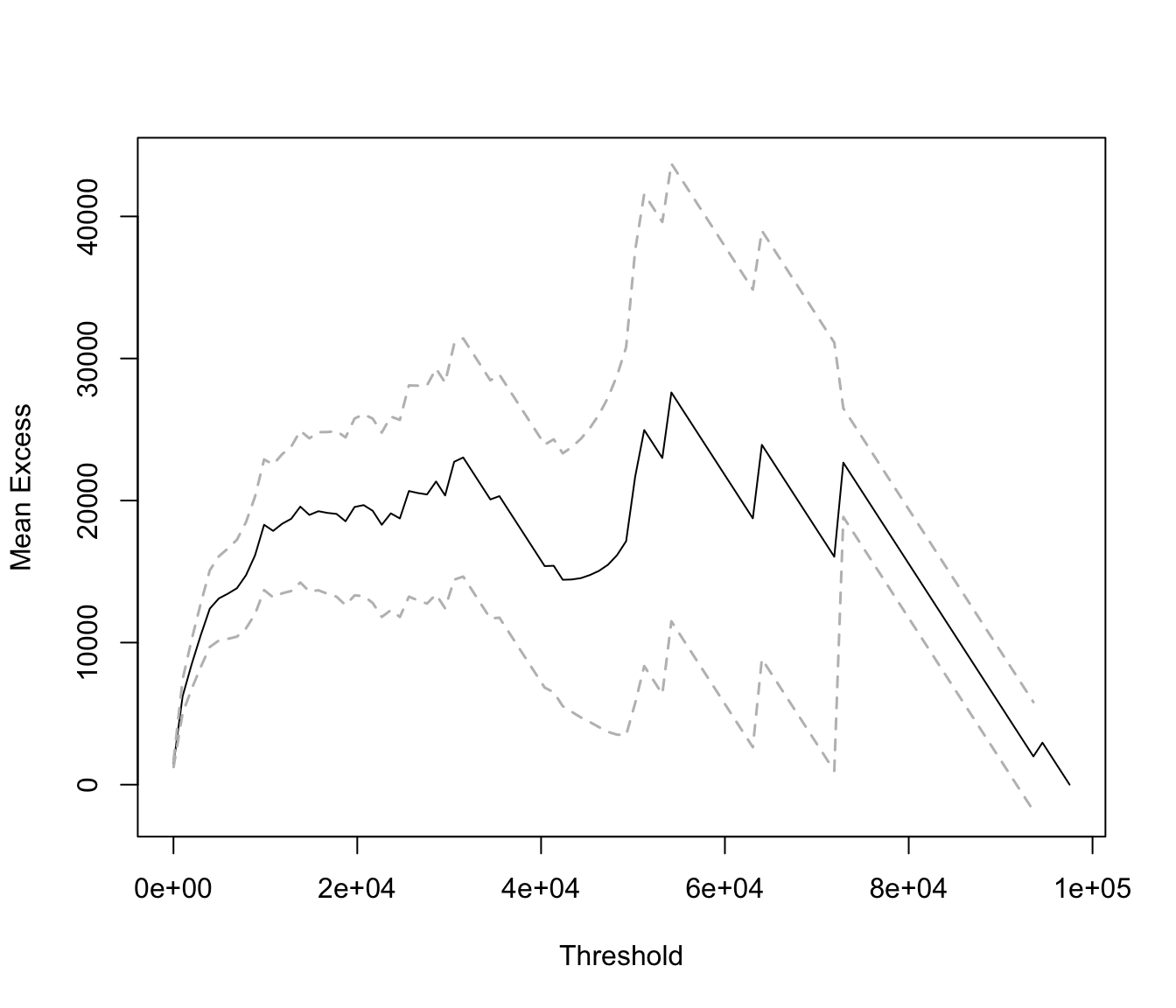
Linear increases point towards a heavy tailed distribution. Here the
graph is biased because dominated by a few very large claims.
If we restrict the graph to range up to 20000 (which is roughly 99% of the data) we get:
mrlplot(SUVA$medcosts[SUVA$medcosts > 0], xlim = c(250, 20000))
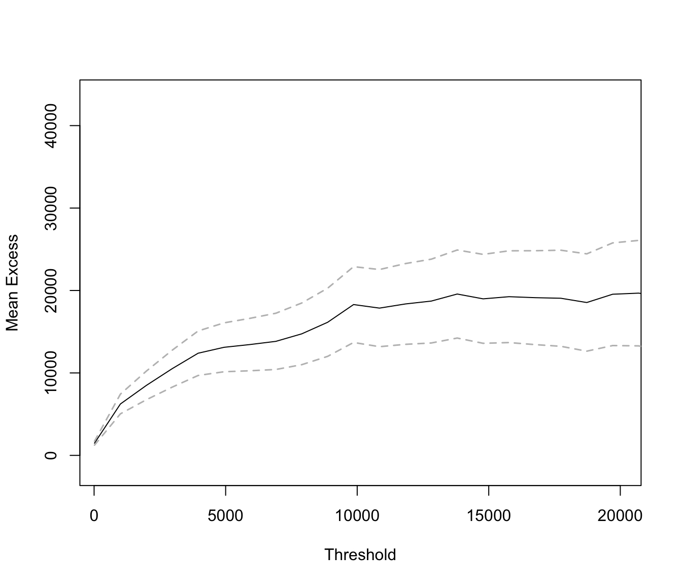
mrlplot(SUVA$dailyallow[SUVA$dailyallow > 0])
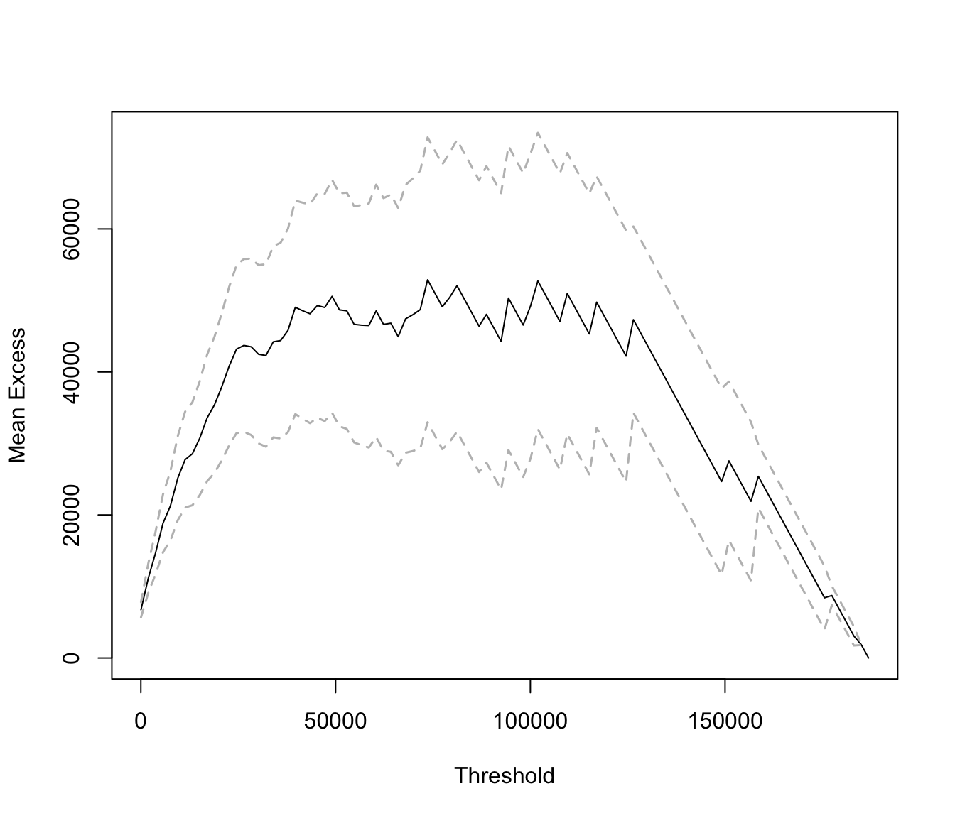
This is not as heavy tailed.
Quantiles #
quantile(SUVA$dailyallow[SUVA$dailyallow > 0])
##       0%      25%      50%      75%     100%
##     26.0    842.0   1763.0   4841.5 186850.0
One can also focus on particular quantiles:
quantile(SUVA$dailyallow[SUVA$dailyallow > 0], probs = c(0.75,
  0.95, 0.99))
##     75%     95%     99%
##  4841.5 25140.5 93285.0
Note this “corresponds” to (crude) empirical versions of Values at Risk (“VaR”s).
(There are better ways of estimating VaRs though.)
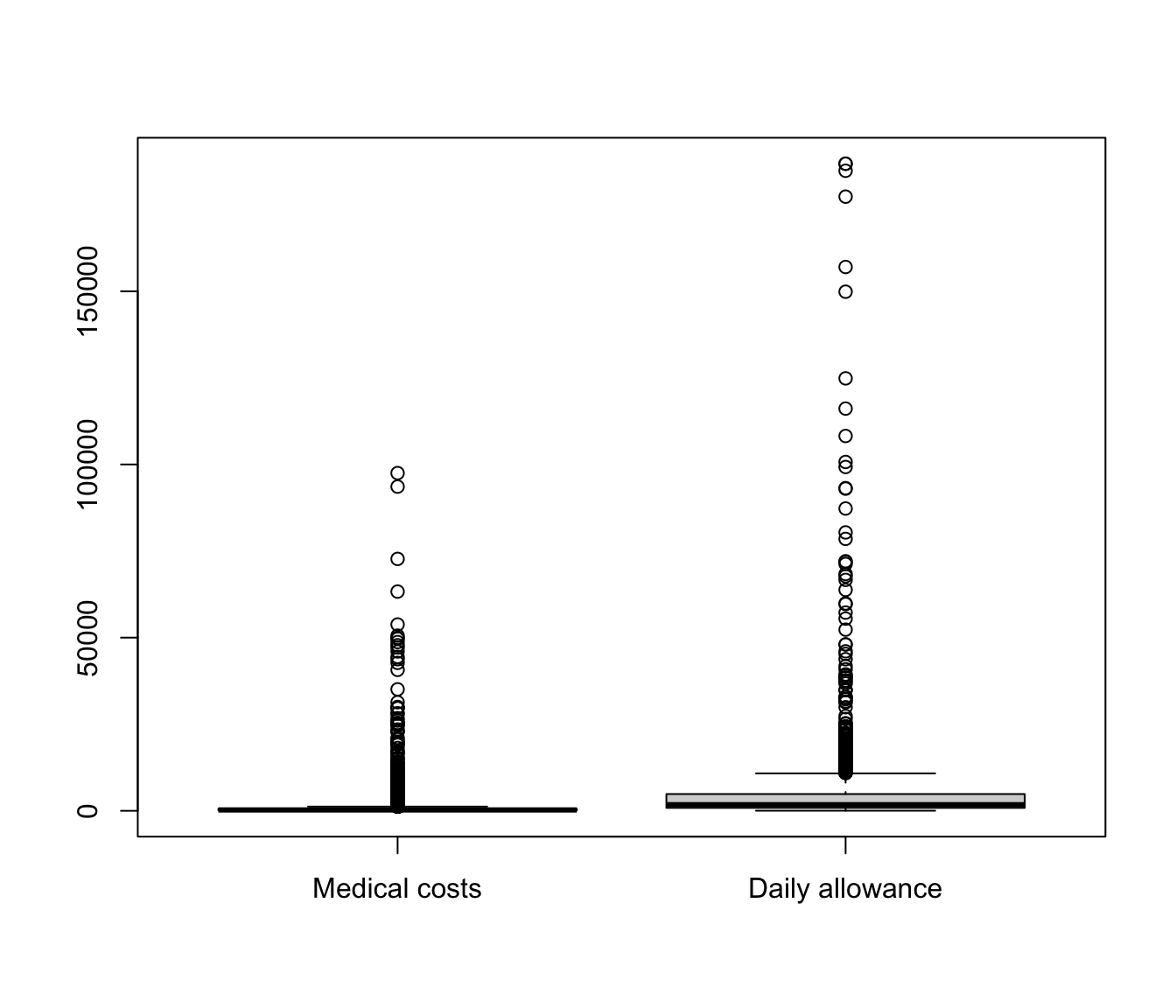
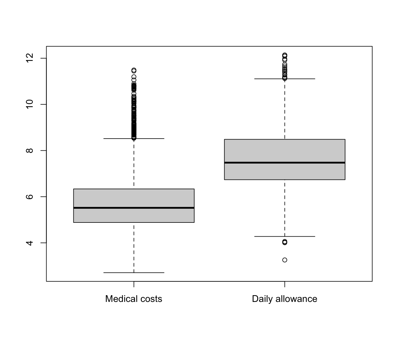
Boxplots #
boxplot(list(`Medical costs` = SUVA$medcosts[SUVA$medcosts >
  0], `Daily allowance` = SUVA$dailyallow[SUVA$dailyallow >
  0]))
boxplot(list(`Medical costs` = log(SUVA$medcosts[SUVA$medcosts >
  0]), `Daily allowance` = log(SUVA$dailyallow[SUVA$dailyallow >
  0])))
Log-log plots #
The log-log plot is defined as
$$ y \rightarrow \left[ \log y, \log (1-G(y))\right],$$
where \(G\) is simply replaced by \(\hat{G}\) for the empirical version.
Just as for the (empirical) mean-excess plots, a linear behaviour (now decreasing) in the (empirical) log-log plot suggests a heavy-tailed distribution. Typical log-log plots are as in Figure 3.19 of Wuthrich (2023).
SUVA log-log plots #
emplot(SUVA$medcosts[SUVA$medcosts > 0], alog = "xy", labels = TRUE)
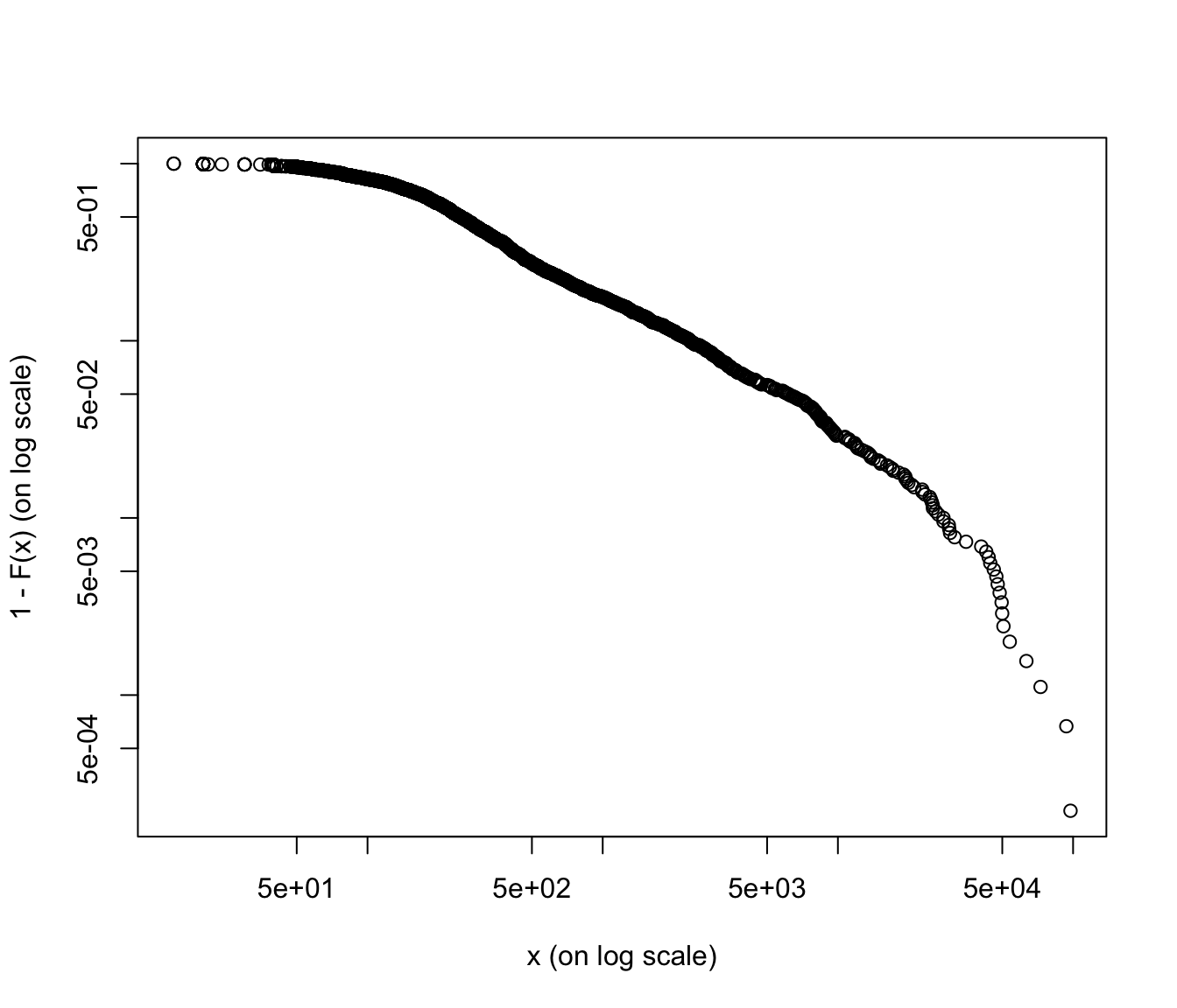
emplot(SUVA$dailyallow[SUVA$dailyallow > 0], alog = "xy", labels = TRUE)
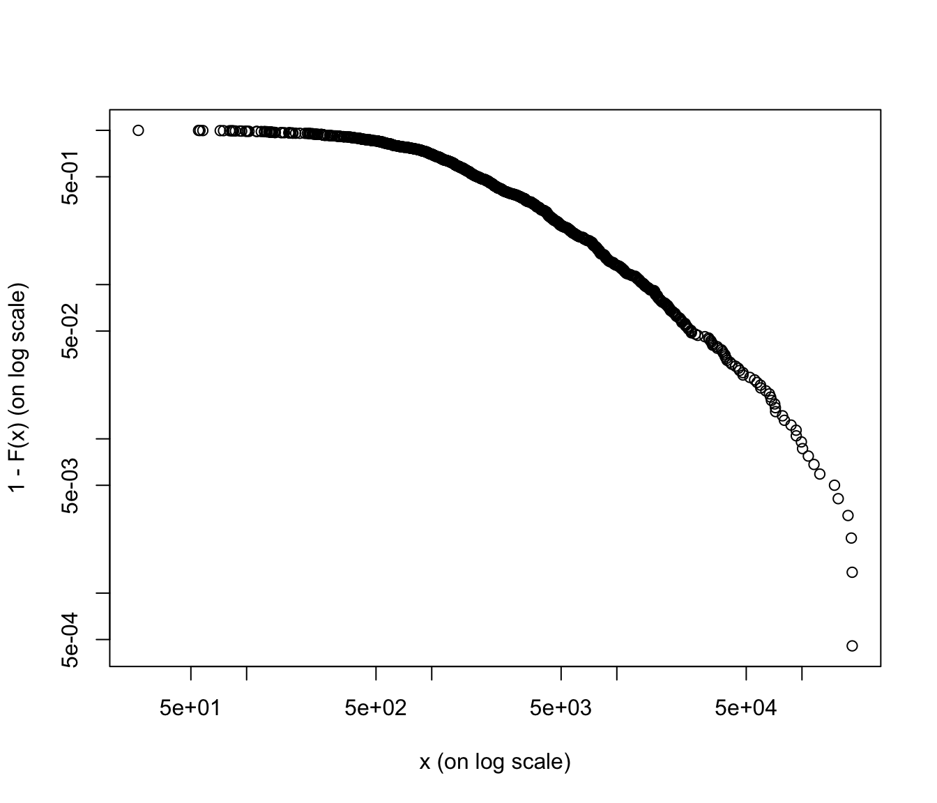
Again, medical costs are a good candidate for heavy tailed distributions (graph is more linear, except at the very end), whereas daily allowance is more reasonably behaved (graph is more concave).
In what follows we will focus on the fitting of daily allowance costs. Medical costs will be modelled in Module 6.
Selected parametric claims size distributions (MW 3.2) #
Parametric models for severity \(Y\)
#
Gamma #
- We shall write
\(Y\sim \Gamma\left( \alpha ,\beta \right)\)if density has the form$$g\left( y\right) =\frac{\beta ^{\alpha }}{\Gamma \left( \alpha \right) }y^{\alpha -1}e^{-\beta y}\text{, for }y>0\text{; }\alpha ,\beta>0\text{.}$$ - Mean:
\(E\left( Y\right) =\alpha /\beta\) - Variance:
\(Var\left( Y\right) =\alpha /\beta ^{2}\) - Skewness:
\(\varsigma_Y=2/\sqrt{\alpha }\)[positively skewed distribution] - Mgf:
\(M_{Y}\left( t\right) =\left( \dfrac{\beta }{\beta-t}\right) ^{\alpha }\), provided\(t < \beta\). - Higher moments:
\(E\left( Y^{k}\right) =\dfrac{\Gamma \left(\alpha +k\right) }{\Gamma \left( \alpha \right) \beta ^{k}}\) - Special case: When
\(\alpha =1\), we have\(Y\sim Exp\left(\beta \right)\)
Inverse Gaussian #
- We shall write
\(Y\sim IG\left( \alpha ,\beta \right)\)if density has the form$$g\left( y\right) =\frac{\alpha y^{-3/2}}{\sqrt{2\pi \beta }}\exp \left[ -\frac{\left( \alpha -\beta y\right) ^{2}}{2\beta y}\right] \text{, for }y>0\text{; }\alpha ,\beta >0\text{.}$$ - Mean:
\(E\left( Y\right) =\alpha / \beta\) - Variance:
\(Var\left( Y\right) =\alpha /\beta ^{2}\) - Skewness:
\(\varsigma_Y=3/\sqrt{\alpha }\)[positively skewed distribution] - Mgf:
\(M_{Y}\left( t\right) =e^{\alpha \left( 1-\sqrt{1-2t/\beta }\right)}\), provided\(t < \beta /2\). - The term “Inverse Gaussian” comes from the fact that there is an inverse relationship between its cgf and that of the Gaussian distribution, but NOT from the fact that the inverse is Gaussian!
Weibull #
- We shall write
\(Y\sim \text{Weibull}\left(\tau,c \right)\)if density has the form$$g\left( y\right) = (c\tau) (cy)^{\tau-1} \exp \{-(cy)^\tau\} \text{, for }y\ge 0\text{; }\alpha ,\beta>0\text{.}$$Note\(G(u)=1-\exp\{-(cy)^\tau\}\). - Mean:
\(E\left( Y\right) =\frac{\gamma(1+1/\tau)}{c}\) - Variance:
\(Var\left( Y\right) =\frac{\gamma(1+2/\tau)}{c^2}-\mu_Y^2\) - Skewness:
\(\varsigma_Y= \left[ \frac{\gamma(1+2/\tau)}{c^2} - 3\mu_Y\sigma_Y^2-\mu_Y^3\right]/ \sigma_Y^3\) - Mgf: does not exist for
\(\tau<1\)and\(t>0\). - Higher moments:
\(E\left( Y^{k}\right) =\frac{\gamma(1+k/\tau)}{c^k}\) - Note: if
\(Z\sim\text{expo}(1)\)then\(Z^{1/\tau}/c\sim \text{Weibull}\left(\tau,c \right)\).
Lognormal #
- We shall write
\(Y\sim \text{LN}\left(\mu, \sigma^2 \right)\)and we have$$\log Y \sim \mathcal{N}(\mu,\sigma^2).$$ - Mean:
\(E\left( Y\right) =\exp\{\mu+\sigma^2/2\}\) - Variance:
\(Var\left( Y\right) =\exp\{2\mu+\sigma^2\}\left(\exp\{\sigma^2\}-1\right)\) - Skewness:
\(\varsigma_Y= \left(\exp\{\sigma^2\}+2\right)\left(\exp\{\sigma^2\}-1\right)^{1/2}\) - Mgf: does not exist for
\(t>0\).
Log-gamma #
- We shall write
\(\log Y\sim \Gamma\left(\gamma, c \right)\)and we have$$g\left( y\right) =\frac{c ^{\gamma }}{\Gamma \left( \gamma \right) }(\log y)^{\gamma -1}y^{-(c+1)}\text{, for }y>0\text{; }\alpha ,\beta>0\text{.}$$ - Mean:
\(E\left( Y\right) =\left(\frac{c}{c-1}\right)^\gamma\)for\(c>1\) - Variance:
\(Var\left( Y\right) =\left(\frac{c}{c-2}\right)^\gamma -\mu_Y^2\)for\(c>2\) - Skewness:
\(\varsigma_Y=\left[ \left(\frac{c}{c-3}\right)^\gamma - 3\mu_Y\sigma_Y^2-\mu_Y^3\right]/ \sigma_Y^3\) - Mgf: does not exist for
\(t>0\). - Higher moments:
\(E\left( Y^{k}\right) =\left(\frac{c}{c-k}\right)^\gamma\)for\(c>k\) - Special case: When
\(\alpha =1\), we have\(Y\sim Exp\left(\beta \right)\)
Pareto Distribution #
- We shall write
\(Y\sim Pareto\left( \theta, \alpha \right)\)if density has the form$$g\left( y\right) = \frac{\alpha}{\theta}\left(\frac{y}{\theta}\right)^{-(\alpha+1)} \quad\text{for }\alert{y\ge \theta}$$ - Mean:
\(E\left( Y\right) =\theta \frac{\alpha}{\alpha-1}\),\(\alpha>1\) - Variance:
\(Var\left( Y\right) =\theta^2 \frac{\alpha}{(\alpha-1)^2(\alpha-2)}\),\(\alpha>2\) - Skewness:
\(\varsigma_Y=\frac{2(1+\alpha)}{\alpha-3}\left(\frac{\alpha-2}{\alpha}\right)^{1/2}\),\(\alpha>3\) - Mgf: does not exist for
\(t>0\) - Translated Pareto: distribution of
\(Y=Y-\beta\)
Extreme Value Theory #
Note that the following topics (which appear briefly in MW 3) will be covered in Module 6 on Extreme Value Theory:
- regular variation at infinity and tail index (page 58-59+)
- Hill plot (page 75+)
- Generalised Pareto (“GP”) and Generalised Extreme Value (“GEV”) distributions
Fitting of distributions (MW3.2) #
Introduction #
- By now, the modeller should have identified some candidate parametric distributions for their data set.
- Example: for
SUVA$dailyallow, based on data numerical and graphical explorations, we decided to try gamma, lognormal, and Weibull.
- Example: for
- In order to be able to compare them, that is, assess their goodness of fit (which will be discussed in the next section), one must find numerical values for the parameters of the candidates.
- The parameter values we will choose will depend on some criterion, which the modeller can choose. In some cases, they may even want to follow different approaches and choose which is the one they think works best for their purposes.
- Fitting criteria include:
- moment matching: choose the
\(m\)parameters such that the first\(m\)moments match - maximum likelihood: choose the parameters such that the overall likelihood that the model generated the data is maximal
\(\adv\)maximum goodness: choose the parameters such that some goodness of fit criterion is maximised
- moment matching: choose the
- We will discuss the first two here, and the third after the goodness of fit section (for obvious reasons).
- There are other criteria which we will not discuss in details, such as:
- quantile matching: choose parameters such that empirical quantiles match theoretical quantiles
- least squares: choose parameters such that the “sum of squares” is minimal (this corresponds to maximum likelihood for Gaussian random variables)
- so-called “minimum distance estimation”, which minimises distances between certain theoretical and empirical functions; see
actuar::mde. For instance theactuarCramér-von Mises method minimises the (weighted) distance between empirical and theoretical cdf’s - score functions such as considered in probabilistic forecasting; see, e.g., package
scoringRulesin Jordan, Krüger, and Lerch (2019)
R and technical notes #
- The function
MASS::fitdistis standard, and uses by default MLE via theoptimfunction. - The package
fitdistrplusallows other fitting criteria (such as method of moments and maximum goodness), and also allows for the user to supply their own optimisation function. - Distributions are coded in the following way. For distribution
foo:dfoois the density (pdf) offoopfoois the distribution function (cdf) offooqfoois the quantile function offoorfoois the random number generator offoo
-
This linkprovides a very comprehensive list of available distributions in R. As a user you can define any distribution yourself, and this syntax will be recognised by some functions. - The package
actuarprovides additional distributions. It also automates the transformation of such distribution functions
in presence of left-truncation and right-censoring (more later).
Moment matching estimation (MME) #
- This is quite straightforward; for a distribution of
\(m\)parameters:- choose
\(m\)moments you care about (usually the first\(m\)moments around the origin or the mean); - build a system of
\(m\)equations (for the\(m\)parameters) matching empirical moments of your choice; - solve the system (might require a computer or some numerical techniques if the equations are not linear).
- choose
- In R, set the argument
methodtommein the call tofitdist- For distributions of 1 and 2 parameters, mean and variances are matched
- For a certain number of distributions a closed form formula is used. For the others, equations are solved numerically using
optimand by minimising the sum of squared differences between theoretical and observed moments.
MME for SUVA #
fit.lnorm.mme <- fitdist(log(SUVA$dailyallow[SUVA$dailyallow >
  0]), "lnorm", method = "mme", order = 1:2)
fit.lnorm.mme$estimate
##   meanlog     sdlog
## 2.0146490 0.1871132
fit.lnorm.mme$loglik
## [1] -1959.06
fit.lnorm.mme2 <- fitdistrplus::mmedist(log(SUVA$dailyallow[SUVA$dailyallow >
  0]), "lnorm", order = 1:2)
fit.lnorm.mme2$estimate
##   meanlog     sdlog
## 2.0146490 0.1871132
fit.lnorm.mme2$loglik
## [1] -1959.06
fit.gamma.mme <- fitdist(log(SUVA$dailyallow[SUVA$dailyallow >
  0]), "gamma", method = "mme", order = 1:2)
fit.gamma.mme$estimate
##     shape      rate
## 28.065081  3.678009
fit.gamma.mme$loglik
## [1] -1951.838
# function to calculate sample raw moment
memp <- function(x, order) emm(x, order)
fit.weibull.mme <- fitdist(log(SUVA$dailyallow[SUVA$dailyallow >
  0]), "weibull", method = "mme", memp = memp, order = c(1,
  2))
fit.weibull.mme$estimate
##    shape    scale
## 6.172910 8.212158
fit.weibull.mme$loglik
## [1] -2020.119
Maximum likelihood estimation (MLE) #
- The likelihood for a statistical model gives an indication of how likely it is that this data set was generated, should the model be correct.
- If there is no censoring or truncation, we have
Obviously, this is a function of the parameter (vector)
\(\mathbf{\theta }=\left( \theta _{1},...,\theta_{m}\right)\), for a given set of observations, denoted\(\mathbf{x}=\left(x_{1},...,x_{n}\right)\). - The value
\(\widehat{\mathbf{\theta }}\)that maximises the likelihood is called the maximum likelihood estimator (MLE). - Often, it is more convenient to maximise the log-likelihood function given by
This avoids issues of underflow for
\(L\)when\(n\)is large.
Note:
- The formulation of a likelihood in presence of left-tuncation and right-censoring will be covered in a later section.
- Sometimes, MLEs match MMEs (check book).
- MLEs have nice properties (such as asymptotic normality, which is one way to estimate standard errors; see later).
MLE for SUVA #
fit.lnorm.mle <- fitdist(log(SUVA$dailyallow[SUVA$dailyallow >
  0]), "lnorm", method = "mle")
fit.lnorm.mle$estimate
##   meanlog     sdlog
## 2.0140792 0.1918442
fit.lnorm.mle$loglik
## [1] -1958.359
fit.gamma.mle <- fitdist(log(SUVA$dailyallow[SUVA$dailyallow >
  0]), "gamma")
fit.gamma.mle$estimate
##     shape      rate
## 27.825788  3.646718
fit.gamma.mle$loglik
## [1] -1951.818
fit.weibull.mle <- fitdist(log(SUVA$dailyallow[SUVA$dailyallow >
  0]), "weibull", method = "mle")
fit.weibull.mle$estimate
##    shape    scale
## 5.527347 8.231313
fit.weibull.mle$loglik
## [1] -2003.26
summary(fit.weibull.mle)
## Fitting of the distribution ' weibull ' by maximum likelihood
## Parameters :
##       estimate Std. Error
## shape 5.527347 0.12127037
## scale 8.231313 0.04760155
## Loglikelihood:  -2003.26   AIC:  4010.519   BIC:  4020.524
## Correlation matrix:
##           shape     scale
## shape 1.0000000 0.3301744
## scale 0.3301744 1.0000000
Parameter uncertainty #
- The estimation of parameters is not perfect.
- The mere fact that different methods lead to different estimates makes that point obvious.
- This will always be true even if we are fitting the right distribution, just because we have only a finite sample of data
- How far can we be from the “truth” ?
- There are different ways of answering that question, two of which we discuss here:
- the Wald approximation: standard errors via the Hessian for MLEs
- bootstrap
Hessian matrix #
The score (or gradient) vector consists of first derivatives
$$S\left( \mathbf{\theta };\mathbf{x}\right) =\left( \frac{\partial \ell \left( \mathbf{\theta };\mathbf{x}\right) }{\partial \theta_{1}},...,\frac{\partial \ell \left( \mathbf{\theta };\mathbf{x}\right) }{\partial \theta_{m}}\right) ^{\prime },$$
so that the MLE satisfies F.O.C. \(S\left(\widehat{\mathbf{\theta}};\mathbf{ x}\right) =\mathbf{0=}\left(0,...,0\right)^{\prime}\).
-
The
\(m\times m\)Hessian matrix for\(\ell\left(\mathbf{\theta};\mathbf{x}\right)\)is defined by$$H\left( \mathbf{\theta };\mathbf{x}\right) =\frac{\partial ^{2}\ell \left( \mathbf{\theta };\mathbf{x}\right) }{\partial \mathbf{\theta}\partial \mathbf{\theta }^{\prime }} =\begin{bmatrix} \dfrac{\partial ^{2}\ell \left( \mathbf{\theta };\mathbf{x}\right)}{\partial \theta _{1}^{2}} & \cdots & \dfrac{\partial ^{2}\ell \left(\mathbf{\theta };\mathbf{x}\right) }{\partial \theta _{1}\partial\theta _{m}} \\ \vdots & \ddots & \vdots \\ \dfrac{\partial ^{2}\ell \left( \mathbf{\theta };\mathbf{x}\right) }{\partial \theta _{m}\partial \theta _{1}} & \cdots & \dfrac{\partial^{2}\ell \left( \mathbf{\theta };\mathbf{x}\right) }{\partial \theta_{m}^{2} } \end{bmatrix}.$$ -
This Hessian is used to estimate
\(Var\left(\widehat{\mathbf{\theta}}\right)\). -
Minus the expected value of this is called the (expected) Fisher information.
The Wald approximation #
It is well-known that a consistent estimator for the covariance matrix \(Var\left(\widehat{\mathbf{\theta}}\right)\) is given by the inverse of the negative of this Hessian matrix:
$$\text{Var}\left(\widehat{\mathbf{\theta}}\right)\ge \widehat{\text{Var}}\left( \widehat{\mathbf{\theta }}\right) =\left[-\mathbf{E}[H\left( \widehat{\mathbf{\theta }};\mathbf{x}\right) ]\right] ^{-1}.$$
The square root of the diagonal elements of this covariance estimate give the standard errors of the MLE estimates. Note:
- “Consistent” means it converges in probability to the value being estimated.
- When
\(n\rightarrow \infty\), the distribution of\(\hat{\theta}\)is asymptotically normal. - Note these are asymptotic results. Furthermore, their quality also strongly depends on the data, the distribution, and the parametrisation of the distribution.
Standard errors for SUVA data #
Note these are obviously unavailable for MMEs. For MLEs:
fit.lnorm.mle$sd
##     meanlog       sdlog
## 0.005786951 0.004091492
summary(fit.lnorm.mle)
## Fitting of the distribution ' lnorm ' by maximum likelihood
## Parameters :
##          estimate  Std. Error
## meanlog 2.0140792 0.005786951
## sdlog   0.1918442 0.004091492
## Loglikelihood:  -1958.359   AIC:  3920.717   BIC:  3930.722
## Correlation matrix:
##         meanlog sdlog
## meanlog       1     0
## sdlog         0     1
fit.gamma.mle$sd
##     shape      rate
## 1.1799866 0.1560432
summary(fit.gamma.mle)
## Fitting of the distribution ' gamma ' by maximum likelihood
## Parameters :
##        estimate Std. Error
## shape 27.825788  1.1799866
## rate   3.646718  0.1560432
## Loglikelihood:  -1951.818   AIC:  3907.636   BIC:  3917.641
## Correlation matrix:
##         shape    rate
## shape 1.00000 0.99103
## rate  0.99103 1.00000
fit.weibull.mle$sd
##      shape      scale
## 0.12127037 0.04760155
summary(fit.weibull.mle)
## Fitting of the distribution ' weibull ' by maximum likelihood
## Parameters :
##       estimate Std. Error
## shape 5.527347 0.12127037
## scale 8.231313 0.04760155
## Loglikelihood:  -2003.26   AIC:  4010.519   BIC:  4020.524
## Correlation matrix:
##           shape     scale
## shape 1.0000000 0.3301744
## scale 0.3301744 1.0000000
\(\adv\) Bootstrap
#
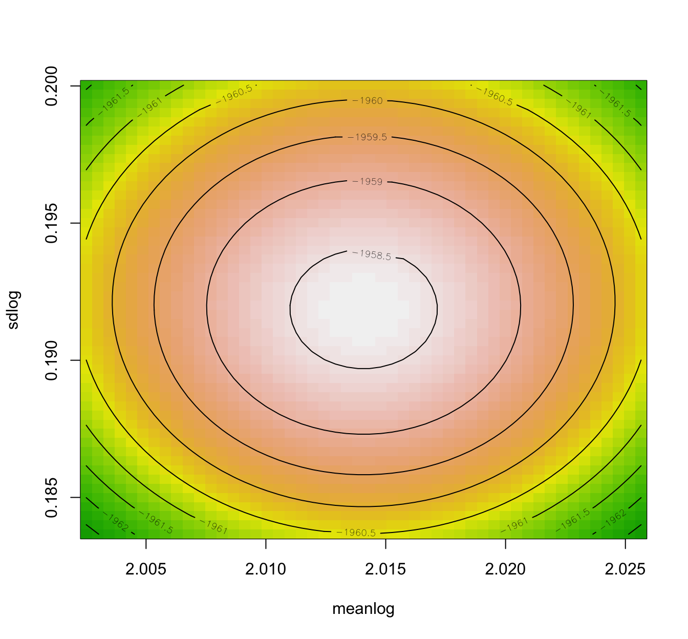
- It is advisable to compare the Wald approximation to the ones obtained using bootstrap procedures.
- Also, the Wald approximation assumes elliptical loglikelihood contours (related to the Gaussian asymptotic result), and hence having a look at the loglikelihood contours is also informative.
- More generally, one might want to simply use bootstrap to compute confidence intervals on parameters (or any function of those parameters).
- In R:
llplotwill provide the loglikelihood contours; andbootdistwill provide bootstrap results on a fitted object.
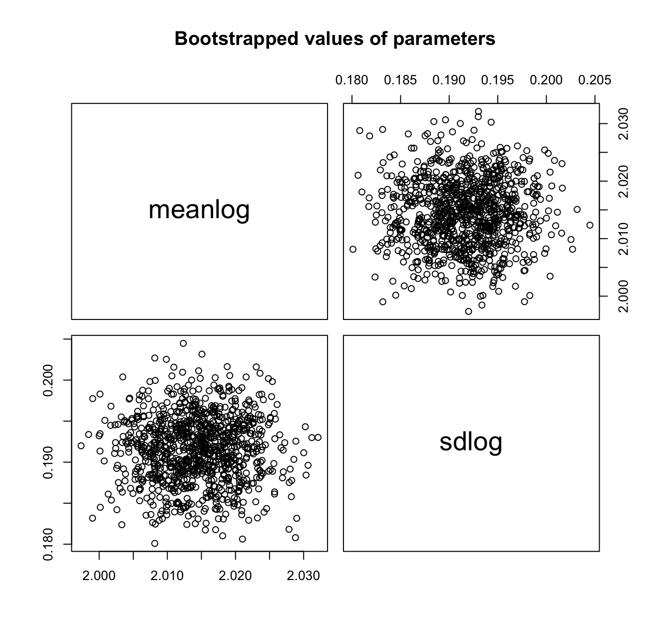
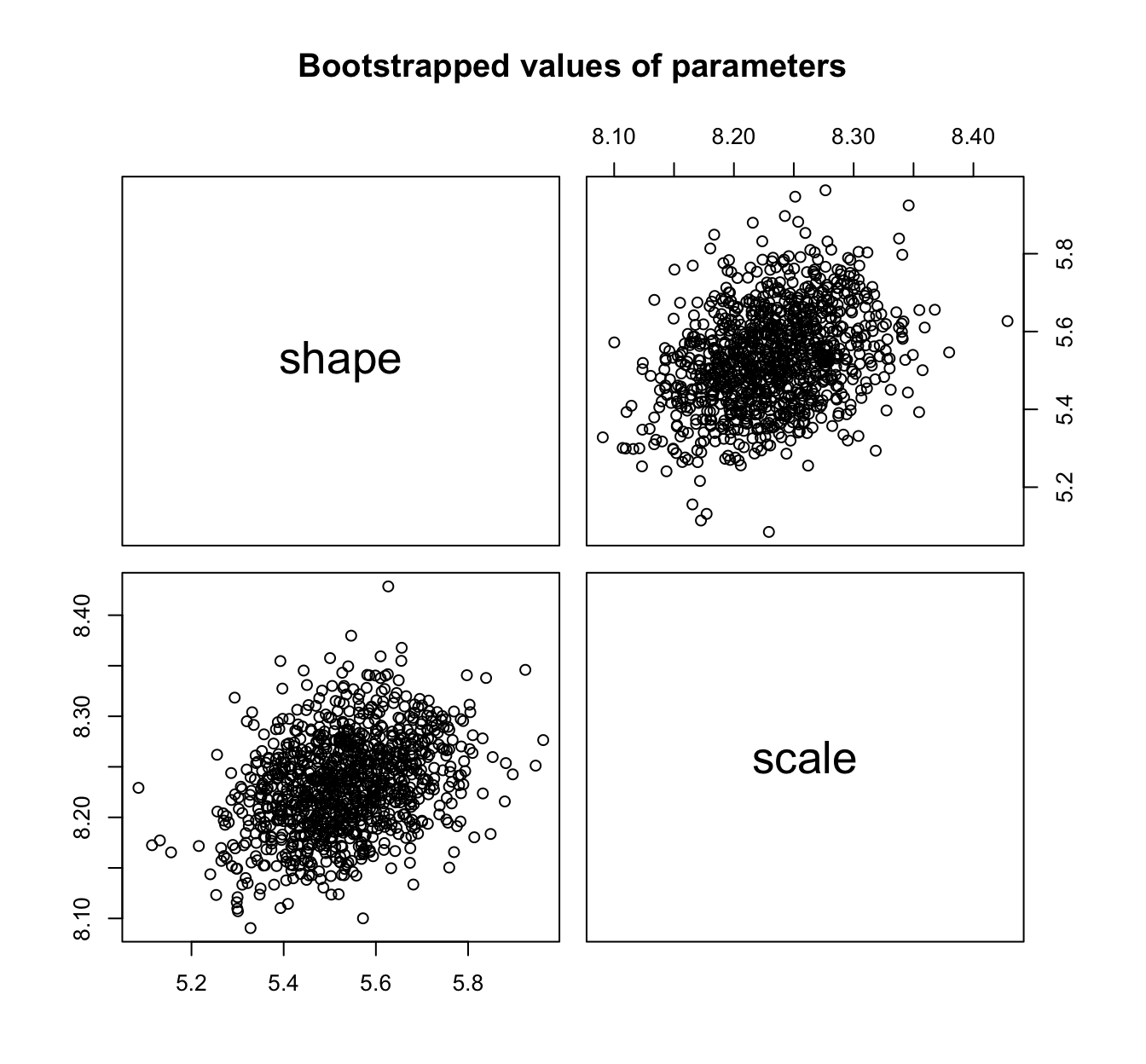
\(\adv\) SUVA contours and bootstrap results
#
llplot(fit.lnorm.mle)
fit.lnorm.mle.boot <- bootdist(fit.lnorm.mle, niter = 1001)
fit.lnorm.mle.boot$fitpart  # the Wald approximation
## Fitting of the distribution ' lnorm ' by maximum likelihood
## Parameters:
##          estimate  Std. Error
## meanlog 2.0140792 0.005786951
## sdlog   0.1918442 0.004091492
summary(fit.lnorm.mle.boot)
## Parametric bootstrap medians and 95% percentile CI
##            Median      2.5%     97.5%
## meanlog 2.0145381 2.0031448 2.0257344
## sdlog   0.1917949 0.1835911 0.1990937
# CI to be compared with
fit.lnorm.mle$estimate + cbind(estimate = 0, `2.5%` = -1.96 *
  fit.lnorm.mle$sd, `97.5%` = 1.96 * fit.lnorm.mle$sd)
##          estimate      2.5%     97.5%
## meanlog 2.0140792 2.0027368 2.0254216
## sdlog   0.1918442 0.1838249 0.1998635
plot(fit.lnorm.mle.boot)
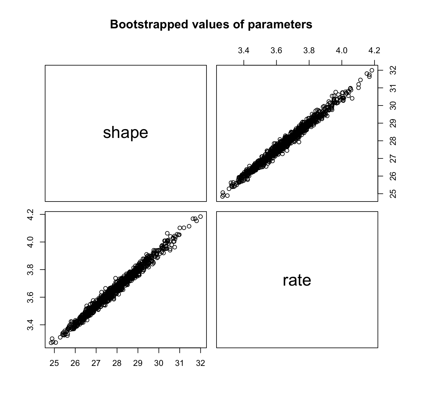
llplot(fit.gamma.mle)
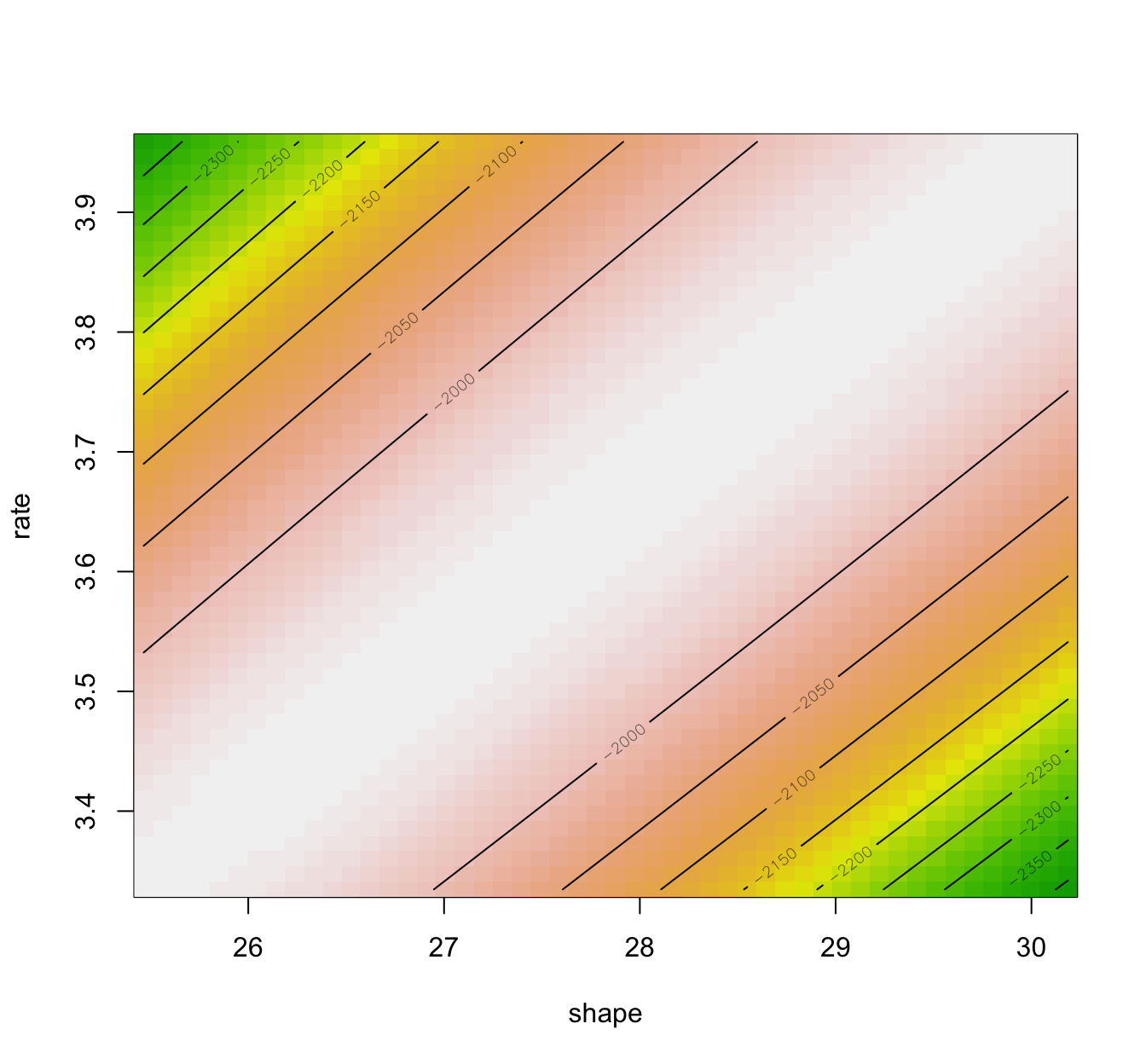
fit.gamma.mle.boot <- bootdist(fit.gamma.mle, niter = 1001)
fit.gamma.mle.boot$fitpart  # the Wald approximation
## Fitting of the distribution ' gamma ' by maximum likelihood
## Parameters:
##        estimate Std. Error
## shape 27.825788  1.1799866
## rate   3.646718  0.1560432
summary(fit.gamma.mle.boot)
## Parametric bootstrap medians and 95% percentile CI
##          Median      2.5%     97.5%
## shape 27.910141 25.795571 30.432601
## rate   3.656702  3.375379  4.003645
# CI to be compared with
fit.gamma.mle$estimate + cbind(estimate = 0, `2.5%` = -1.96 *
  fit.gamma.mle$sd, `97.5%` = 1.96 * fit.gamma.mle$sd)
##        estimate      2.5%     97.5%
## shape 27.825788 25.513015 30.138562
## rate   3.646718  3.340873  3.952562
plot(fit.gamma.mle.boot)
llplot(fit.weibull.mle)
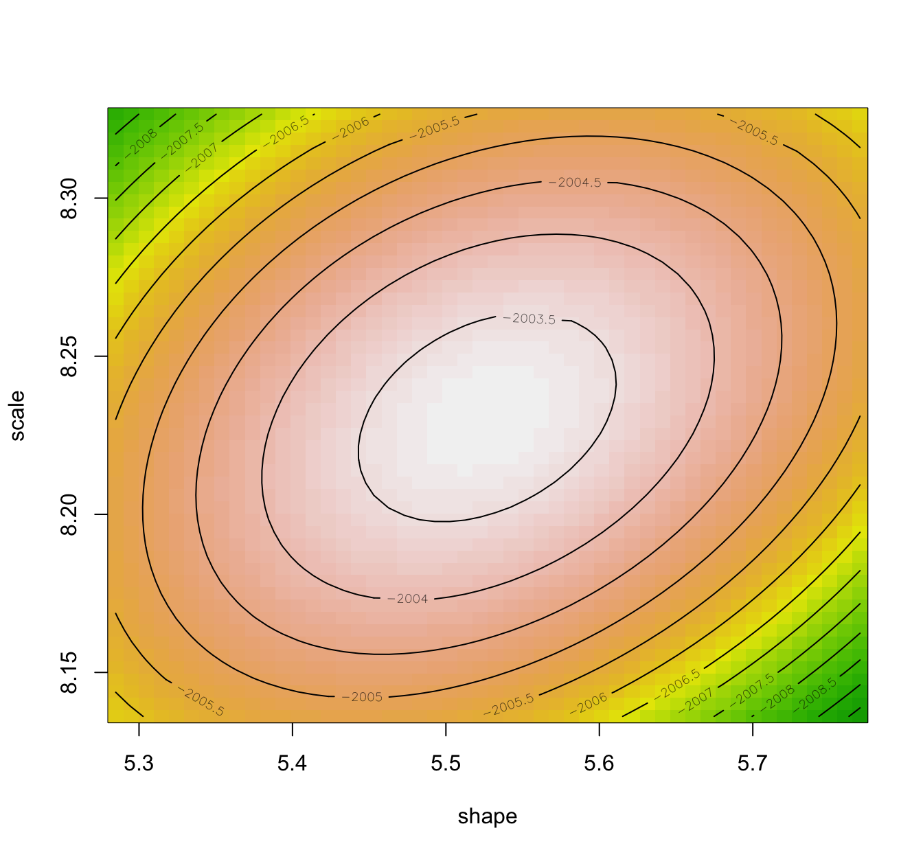
fit.weibull.mle.boot <- bootdist(fit.weibull.mle, niter = 1001)
fit.weibull.mle.boot$fitpart  # the Wald approximation
## Fitting of the distribution ' weibull ' by maximum likelihood
## Parameters:
##       estimate Std. Error
## shape 5.527347 0.12127037
## scale 8.231313 0.04760155
summary(fit.weibull.mle.boot)
## Parametric bootstrap medians and 95% percentile CI
##         Median     2.5%    97.5%
## shape 5.528090 5.297146 5.784021
## scale 8.231434 8.142609 8.327401
# CI to be compared with
fit.weibull.mle$estimate + cbind(estimate = 0, `2.5%` = -1.96 *
  fit.weibull.mle$sd, `97.5%` = 1.96 * fit.weibull.mle$sd)
##       estimate     2.5%    97.5%
## shape 5.527347 5.289657 5.765037
## scale 8.231313 8.138014 8.324612
plot(fit.weibull.mle.boot)
\(\adv\) Confidence intervals on other quantities
#
- One can readily obtain confidence intervals on quantiles with the
quantilefunction and abootdistobject - More generally, this can be done of any function; see Delignette-Muller and Dutang (2015).
quantile(fit.gamma.mle.boot)
## (original) estimated quantiles for each specified probability (non-censored data)
##             p=0.1    p=0.2    p=0.3    p=0.4    p=0.5    p=0.6
## estimate 5.845174 6.394064 6.810817 7.181091 7.539156 7.908945
##             p=0.7   p=0.8    p=0.9
## estimate 8.317716 8.81358 9.532902
## Median of bootstrap estimates
##            p=0.1    p=0.2    p=0.3    p=0.4    p=0.5    p=0.6
## estimate 5.84611 6.396059 6.812535 7.182716 7.539946 7.910672
##             p=0.7    p=0.8    p=0.9
## estimate 8.318227 8.814841 9.533408
##
## two-sided 95 % CI of each quantile
##           p=0.1    p=0.2    p=0.3    p=0.4    p=0.5    p=0.6    p=0.7
## 2.5 %  5.752505 6.308144 6.729508 7.102813 7.459106 7.823908 8.224559
## 97.5 % 5.947397 6.488367 6.897450 7.266903 7.626204 7.999964 8.411769
##           p=0.8    p=0.9
## 2.5 %  8.706754 9.401727
## 97.5 % 8.916318 9.661838
Dealing with left-truncation and right-censoring #
Coding of censored data in R #
- We need two columns named
leftandright. - The
leftcolumn contains:NAfor left censored observations- the left bound of the interval for interval censored observations
- the observed value for non-censored observations
- The
rightcolumn contains:NAfor right censored observations- the right bound of the interval for interval censored observations
- the observed value for non-censored observations
- This corresponds to the coding names
interval2in functionSurvof the packagesurvival
In other words, (left,right) corresponds to
(a,a)for an exact observation ata($=a$)(a,NA)for a right censored observation ata($>a$)(NA,b)for a left censored observation atb($\le b$)(a,b)for an interval censored observation over\((a,b)\), where\(b>a\)($>a$ and\(\le b\))
For example, consider twenty values from the canlifins of the CASdatasets package (see Delignette-Muller and Dutang (n.d.))
exitage <- c(81.1, 78.9, 72.6, 67.9, 60.1, 78.3, 83.4, 66.9,
  74.8, 80.5, 75.6, 67.1, 75.3, 82.8, 70.1, 85.4, 74, 70, 71.6,
  76.5)
death <- c(0, 0, 1, 0, 0, 0, 0, 1, 0, 0, 0, 0, 0, 0, 1, 1, 0,
  0, 0, 0)
- the first value is someone who exited the study at 81.1, but not via death, so it is a right-censored observation
- this needs to be coded:
left: 81.1right:NA
Overall, this becomes:
casdata <- cbind.data.frame(left = exitage, right = exitage)
casdata$right[death == 0] <- NA  # the censored values
print(casdata)
##    left right
## 1  81.1    NA
## 2  78.9    NA
## 3  72.6  72.6
## 4  67.9    NA
## 5  60.1    NA
## 6  78.3    NA
## 7  83.4    NA
## 8  66.9  66.9
## 9  74.8    NA
## 10 80.5    NA
## 11 75.6    NA
## 12 67.1    NA
## 13 75.3    NA
## 14 82.8    NA
## 15 70.1  70.1
## 16 85.4  85.4
## 17 74.0    NA
## 18 70.0    NA
## 19 71.6    NA
## 20 76.5    NA
(Note: How to use the function Surv() is explained in Delignette-Muller and Dutang, n.d.)
Censored data can be plotted raw…
plotdistcens(casdata, NPMLE = FALSE)
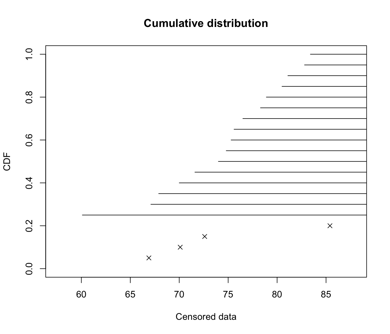
… or as an empirical distribution
plotdistcens(casdata)
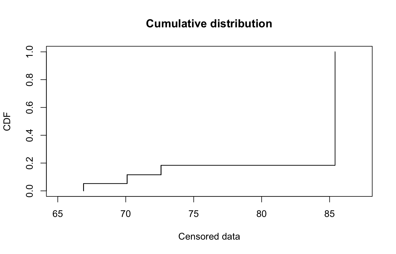
Note that there are some technical subtleties with creating empirical distributions for censored data. This is out of scope, but details can be found in Delignette-Muller and Dutang (n.d.), Delignette-Muller and Dutang (2015), and references therein.
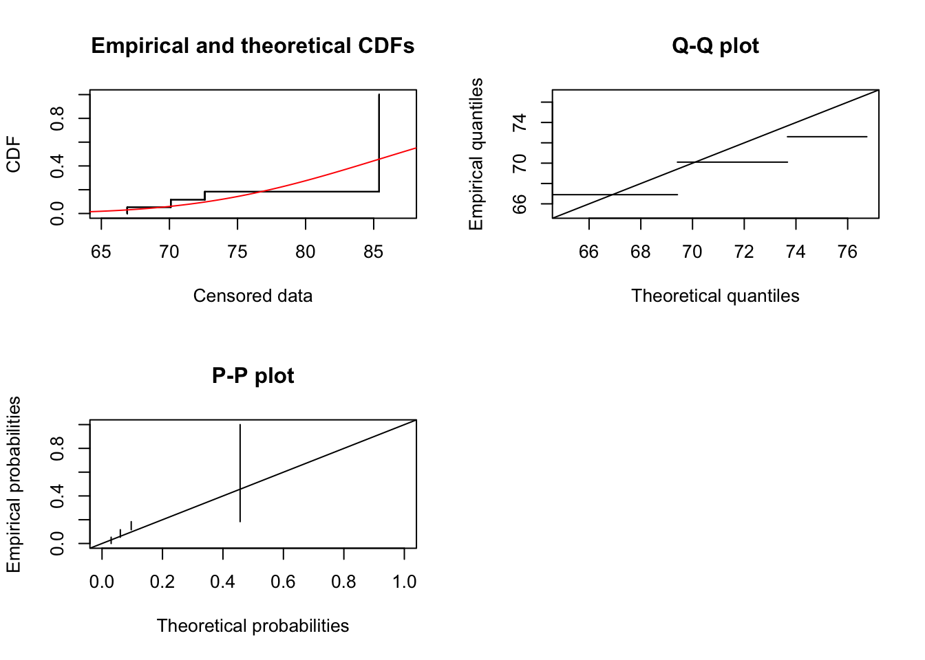
Fitting censored data #
- Again, this is easily done with associated
foocensfunctions
cas.gamma.fit <- fitdistcens(casdata, "gamma")
summary(cas.gamma.fit)
## Fitting of the distribution ' gamma ' By maximum likelihood on censored data
## Parameters
##         estimate Std. Error
## shape 57.7413639 41.0307481
## rate   0.6626575  0.5056786
## Loglikelihood:  -20.0179   AIC:  44.0358   BIC:  46.02727
## Correlation matrix:
##           shape      rate
## shape 1.0000000 0.9983071
## rate  0.9983071 1.0000000
- Commands like
cdfcompcensbootdistcensalso exist. - However,
gofstatis not available as there do not exist results general enough to be coded in the package. Specific results for right-censored variables do exist, though.
plot(cas.gamma.fit)
Left-truncation and R #
- Unfortunately there is no pre-coded function for left-truncation.
- It can be done manually, with care.
- With left-truncation, the key (from definition) is that an observation will exist, if, and only if, it was beyond the truncation point. This means that the probability/likelihood associated to each observation is conditional on it being more than the truncation point.
- What follows is generalised to left- and right- truncation, and is taken from Delignette-Muller and Dutang (n.d.).
- For
\(X\)before truncation, the\(l\)-left-truncated,\(u\)-right-truncated variable\(Y\)has density$$g_Y(y)= \left\{ \begin{array}{cl} \frac{g_X(x)}{G_X(u)-G_X(l)} & \text{if }l<x<u \\ 0 & \text{otherwise} \end{array} \right.$$
As an example in R, the d and p functions of a truncated exponential can be coded as:
dtexp <- function(x, rate, low, upp) {
  PU <- pexp(upp, rate = rate)
  PL <- pexp(low, rate = rate)
  dexp(x, rate)/(PU - PL) * (x >= low) * (x <= upp)
}
ptexp <- function(q, rate, low, upp) {
  PU <- pexp(upp, rate = rate)
  PL <- pexp(low, rate = rate)
  (pexp(q, rate) - PL)/(PU - PL) * (q >= low) * (q <= upp) +
    1 * (q > upp)
}
If we generate 200 such truncated variables:
set.seed(22042021)
n <- 200  # number of observations
x <- rexp(n)  # simulating sample of x's
y <- x[x > 0.5 & x < 3]  # truncating to get sample of y's
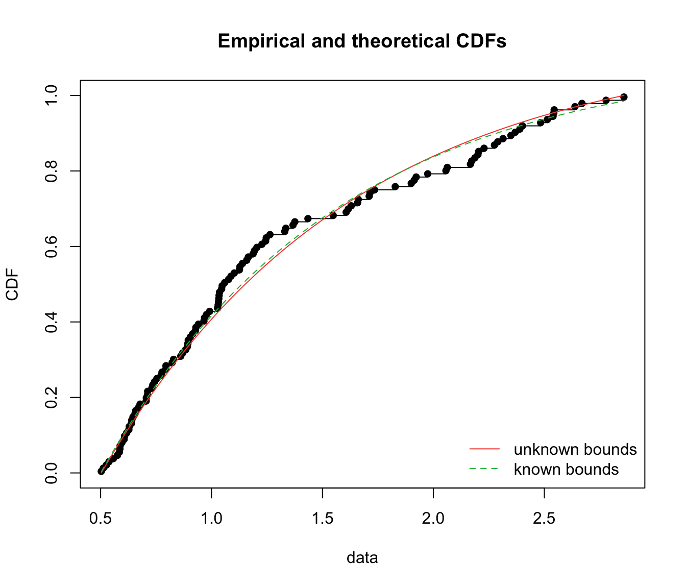
and then fit them with either left- and right- truncation estimated from the data:
fit.texp.emp <- fitdist(y, "texp", method = "mle", start = list(rate = 3),
  fix.arg = list(low = min(y), upp = max(y)))
… or in an informative way (i.e. we know what the bounds are):
fit.texp.inf <- fitdist(y, "texp", method = "mle", start = list(rate = 3),
  fix.arg = list(low = 0.5, upp = 3))
gofstat(list(fit.texp.emp, fit.texp.inf), fitnames = c("unknown bounds",
  "known bounds"))
## Goodness-of-fit statistics
##                              unknown bounds known bounds
## Kolmogorov-Smirnov statistic     0.07546318   0.06747339
## Cramer-von Mises statistic       0.13211330   0.09999122
## Anderson-Darling statistic              Inf   0.59863722
##
## Goodness-of-fit criteria
##                                unknown bounds known bounds
## Akaike's Information Criterion       165.3424     169.7301
## Bayesian Information Criterion       168.1131     172.5007
cdfcomp(list(fit.texp.emp, fit.texp.inf), legendtext = c("unknown bounds",
  "known bounds"))
Likelihood formulation with both left-truncation and right-censoring #
- For our purposes, we shall represent our set of observations as
$$\left( t_{j},x_{j},\delta_{j}\right)$$where\(t_{j}\)is the left truncation point;\(x_{j}\)is the claim value that produced the data point; and\(\delta_{j}\)is indicator whether limit has been reached.
- For example:
\(\left( 50,250,0\right)\)\(\left( 100,1100,1\right)\)
Densities will be as follows:
$$
L\left( \mathbf{\theta };\mathbf{x}\right) =\prod\nolimits_{j}\left[
\frac{ f\left( x_{j};\mathbf{\theta }\right) }{1-F\left(
t_{j};\mathbf{\theta } \right) }\right] ^{1-\delta_{j}}\cdot
\prod\nolimits_{j}\left[ \frac{ 1-F\left( x_{j};\mathbf{\theta
}\right) }{1-F\left( t_{j};\mathbf{\theta } \right) }\right]
^{\delta_{j}}.
$$
The contribution to the likelihood function for a data point where the
limit has not been reached is given by
$$
\left[ \frac{f\left( x_{j}\right) }{1-F\left( t_{j}\right) }\right]
^{1-\delta_{j}}.
$$
The contribution to the likelihood function for a data point where
the limit has been reached is given by
$$
\left[ \frac{1-F\left( x_{j}\right) }{1-F\left( t_{j}\right)
}\right] ^{\delta_{j}}.
$$
Note here that the policy limit if reached would be equal to \(x_{j}-t_{j}\).
When truncation and censoring levels are the same everywhere #
- In R, the approach will be to code a left-truncated function, and then use the
foocensfunctions. - Let us do this on a gamma distribution:
dtgamma <- function(x, rate, shape, low) {
  PL <- pgamma(low, rate = rate, shape = shape)
  dgamma(x, rate = rate, shape = shape)/(1 - PL) * (x >= low)
}
ptgamma <- function(q, rate, shape, low) {
  PL <- pgamma(low, rate = rate, shape = shape)
  (pgamma(q, rate = rate, shape = shape) - PL)/(1 - PL) * (q >=
    low)
}
We initially assume that the truncation and censoring levels are the same everywhere.
For instance,
- truncated at 2
- censored at 20
for all data points.
Simulating one such dataset:
set.seed(22042021)
n <- 2000  # number of observations
x <- rgamma(n, shape = 2, rate = 0.2)  # simulating sample of x's
x <- x[x > 2]  # left-truncation at 2
n - length(x)  # number of observations that were truncated
## [1] 123
censoring <- x > 20  # we will censor at 20
x[x > 20] <- 20  # censoring at 20
Transforming this into the right format:
censoring[censoring == FALSE] <- x[censoring == FALSE]
censoring[censoring == TRUE] <- NA
xcens <- cbind.data.frame(left = x, right = censoring)
And fitting:
# Not allowing for truncation:
fit.gamma.xcens <- fitdistcens(xcens, "gamma", start = list(shape = mean(xcens$left)^2/var(xcens$left),
  rate = mean(xcens$left)/var(xcens$left)))
summary(fit.gamma.xcens)
...
## Fitting of the distribution ' gamma ' By maximum likelihood on censored data
## Parameters
##        estimate  Std. Error
## shape 2.7153083 0.089141065
## rate  0.2566683 0.009500217
## Loglikelihood:  -5412.521   AIC:  10829.04   BIC:  10840.12
...
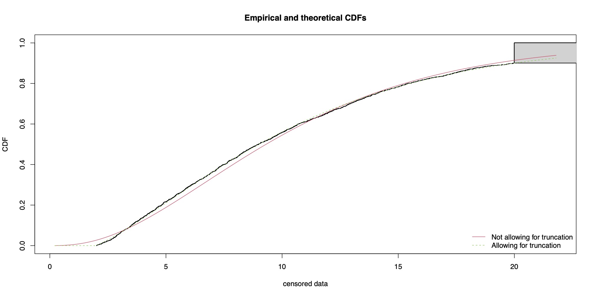
# Allowing for truncation
fit.tgamma.xcens <- fitdistcens(xcens, "tgamma", start = list(shape = mean(xcens$left)^2/var(xcens$left),
  rate = mean(xcens$left)/var(xcens$left)), fix.arg = list(low = min(xcens$left)))
summary(fit.tgamma.xcens)
...
## Fitting of the distribution ' tgamma ' By maximum likelihood on censored data
## Parameters
##        estimate Std. Error
## shape 2.0296237 0.10529978
## rate  0.2006534 0.01009728
## Fixed parameters:
##        value
## low 2.013575
## Loglikelihood:  -5340.151   AIC:  10684.3   BIC:  10695.38
...
cdfcompcens(list(fit.gamma.xcens, fit.tgamma.xcens), legendtext = c("Not allowing for truncation",
  "Allowing for truncation"))
When truncation and censoring levels vary #
In real life, an insurance product would have more than one level of deductibles and limits to suit different policyholders. Simulating another dataset:
set.seed(2022)
n <- 3006  # number of observations 9 x 334
orig_x <- rgamma(n, shape = 2, rate = 0.2)  # simulating sample of x's
deductibles <- rep(c(rep(1, 3), rep(3, 3), rep(5, 3)), 334)
limits <- rep(c(15, 20, 30), 3 * 334) + deductibles
# limit is on payment, not raw loss
Manually applying the deductibles and limits:
x <- orig_x
censored <- x>limits # we will censor at the limits
x[censored] <- limits[censored] # censoring at the limits
# the above takes only elements of x which have TRUE
# in the vector censored
#
deducted <- x > deductibles
x <- x[deducted] # left-truncation at all points
# here the truncated observations disappear!
n-length(x) # observations that were truncated
## [1] 431
# that many were removed
#
claims <- data.frame(x = x, #
                     deduct = deductibles[deducted], #
                     limitI = censored[deducted])
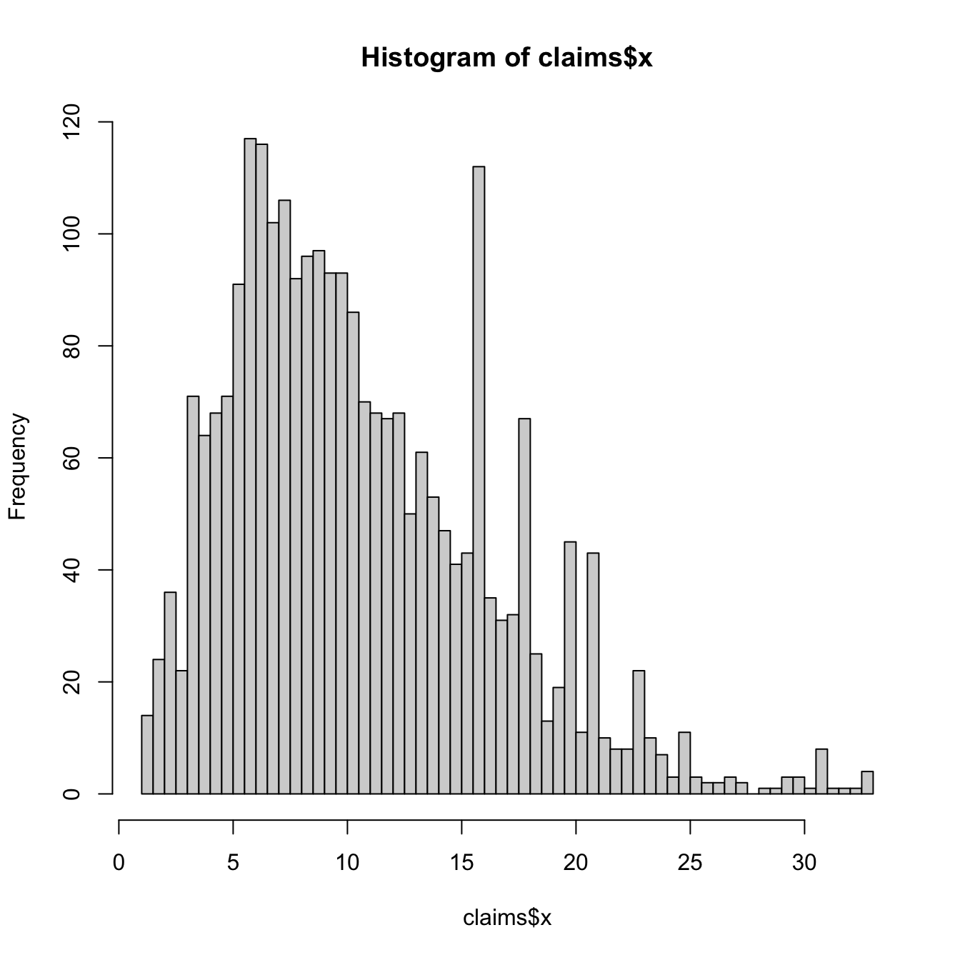
Preliminary analysis:
(note that there are no claims less than 1)
claims <- claims[sample(1:nrow(claims), nrow(claims)), ]  # randomising data
# we pretend we do not know how the data was generated
head(claims)
##              x deduct limitI
## 444  17.196879      1  FALSE
## 1733 13.964488      3  FALSE
## 1414  3.521077      1  FALSE
## 1407 15.488936      1  FALSE
## 1138 11.509672      3  FALSE
## 1977  4.875571      3  FALSE
hist(claims$x, breaks = 100)
# Note this includes right-censored observations But not
# the truncated values
Preparing our joint log-likelihood function:
Here, we are minimising a negative log-likelihood instead of maximising a log-likelihood.
negloglik <- function(pdf, cdf, param, x, deduct, limitI) {
  # Function returns the negative log likelihood of the
  # censored and truncated dataset. Each data point's
  # contribution to the log likelihood depends on the
  # theoretical distribution pdf and cdf and also the
  # deductible and limit values to adjust for truncation
  # and censoring
  PL <- do.call(cdf, c(list(q = deduct), param))
  PX <- do.call(cdf, c(list(q = x), param))
  fX <- do.call(pdf, c(list(x = x), param))
  lik.contr <- ifelse(limitI, log(1 - PX), log(fX)) - log(1 -
    PL)
  return(-sum(lik.contr))
}
Fitting the distribution
Let’s try gamma. Note that our objective function needs starting values for the optimisation. What other starting values could we use?
pdf <- dgamma
cdf <- pgamma
x <- claims$x
deduct <- claims$deduct
limitI <- claims$limitI
# MME for starting values
start <- list(shape = mean(x)^2/var(x), rate = mean(x)/var(x))
obj.fun <- function(shape, rate) {
  param <- list(shape = shape, rate = rate)
  return(negloglik(pdf, cdf, param, x, deduct, limitI))
}  # we now have a function to minimise wrt shape and rate
gamma.ll.fit <- stats4::mle(obj.fun, start = start, lower = c(0,
  0))
summary(gamma.ll.fit)
param.g.ll <- stats4::coef(gamma.ll.fit)
param.g.ll
## Length  Class   Mode
##      1    mle     S4

##     shape      rate
## 2.1297568 0.2111871
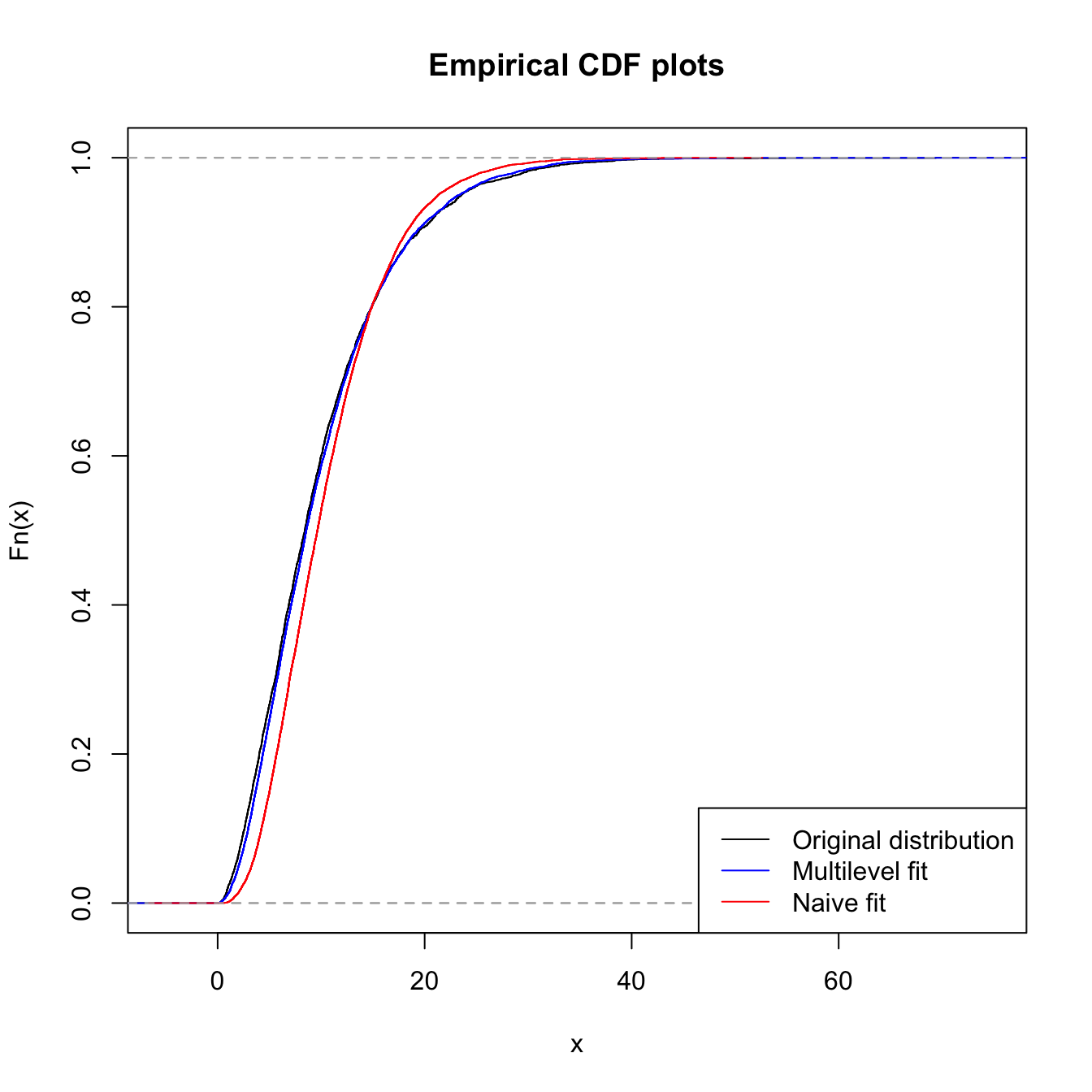
How did we go?
fit.tcens.param <- param.g.ll  # from the proper fit
fit.param <- coef(fitdistrplus::fitdist(claims$x, "gamma", method = "mle"))
# this is a naive fit
sim.tcens.gamma <- rgamma(10000, shape = fit.tcens.param[1],
  rate = fit.tcens.param[2])  # sample from proper fit
sim.gamma <- rgamma(10000, shape = fit.param[1], rate = fit.param[2])
# sample from naive fit
# Comparing the proper fit (that accounts for l-trunc and
# r-cens) with a 'naive' fit (that does not account for
# those)
plot(ecdf(orig_x), main = "Empirical CDF plots", col = "black")
lines(ecdf(sim.tcens.gamma), col = "blue", type = "s")
lines(ecdf(sim.gamma), col = "red", type = "s")
legend("bottomright", legend = c("Original distribution", "Multilevel fit",
  "Naive fit"), lty = 1, col = c("black", "blue", "red"))
Model selection (MW 3.3) #
Graphical approaches #
For judging quality of model, do some graphical comparisons:
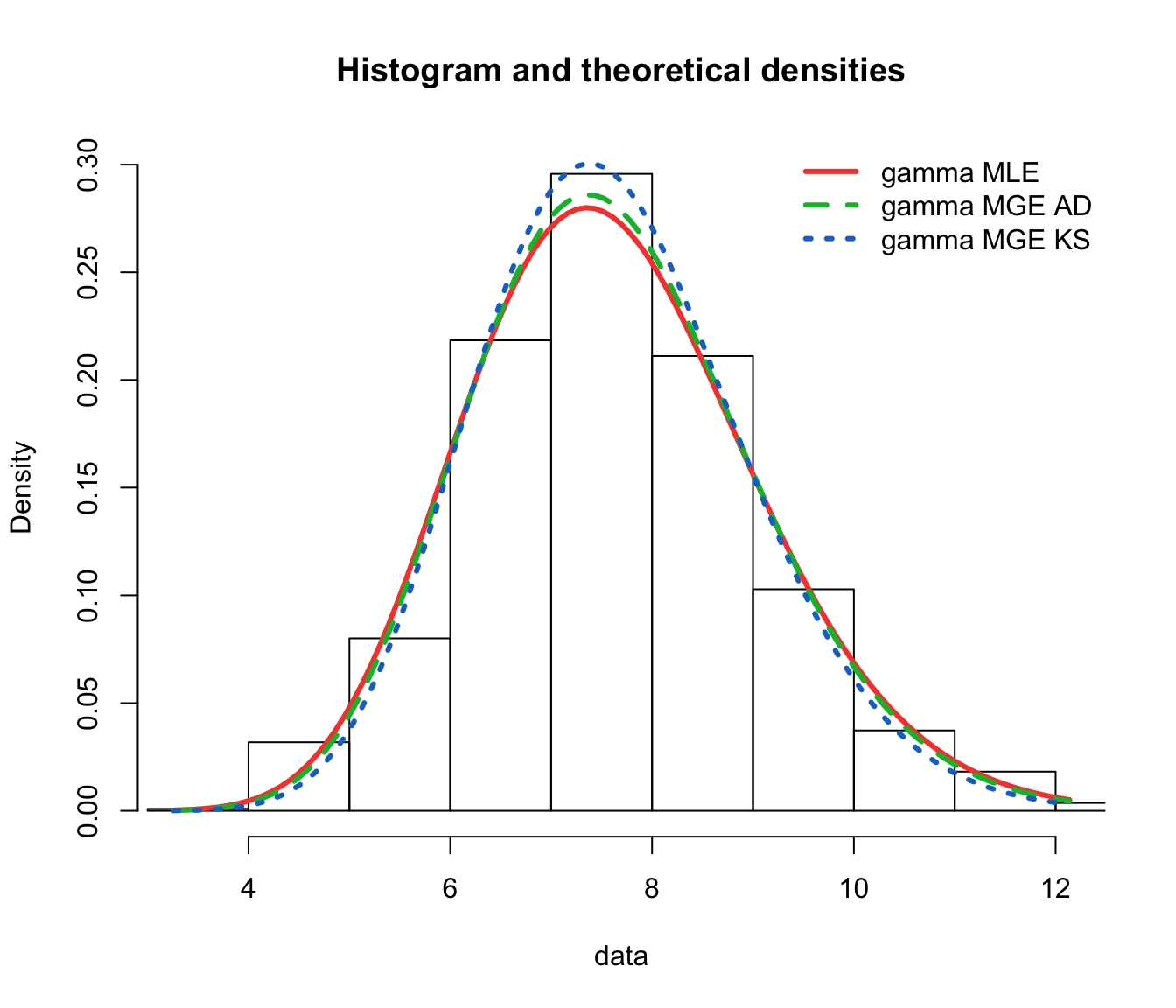
- histogram vs. fitted parametric density function;
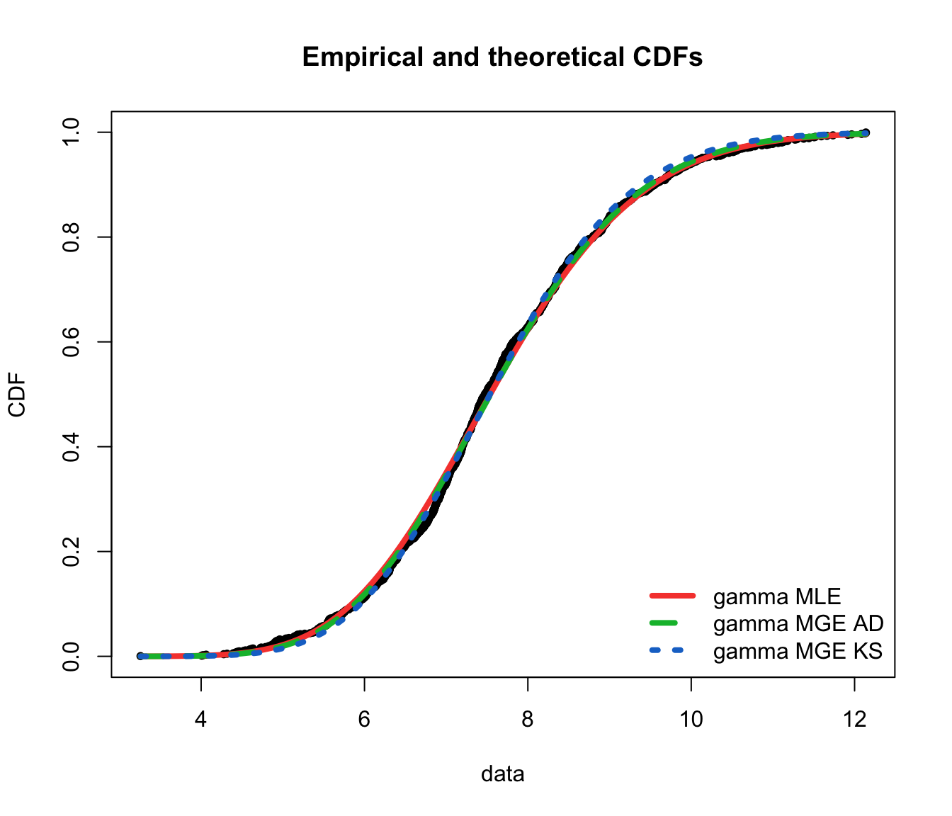
- empirical CDF vs fitted parametric CDF;
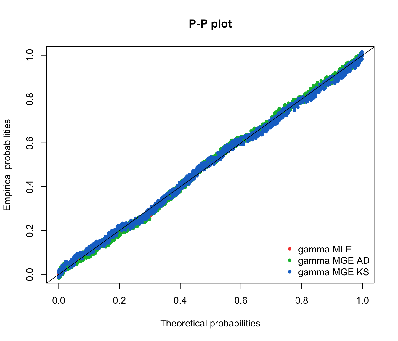
- probability-probability (P-P) plot - theoretical vs empirical cumulative probabilities;
- quantile-quantile (Q-Q) plot - theoretical vs sample quantiles.
Let the (theoretical) fitted parametric distribution be denoted by
\(G\left( x;\widehat{\mathbf{\theta }}\right)\).
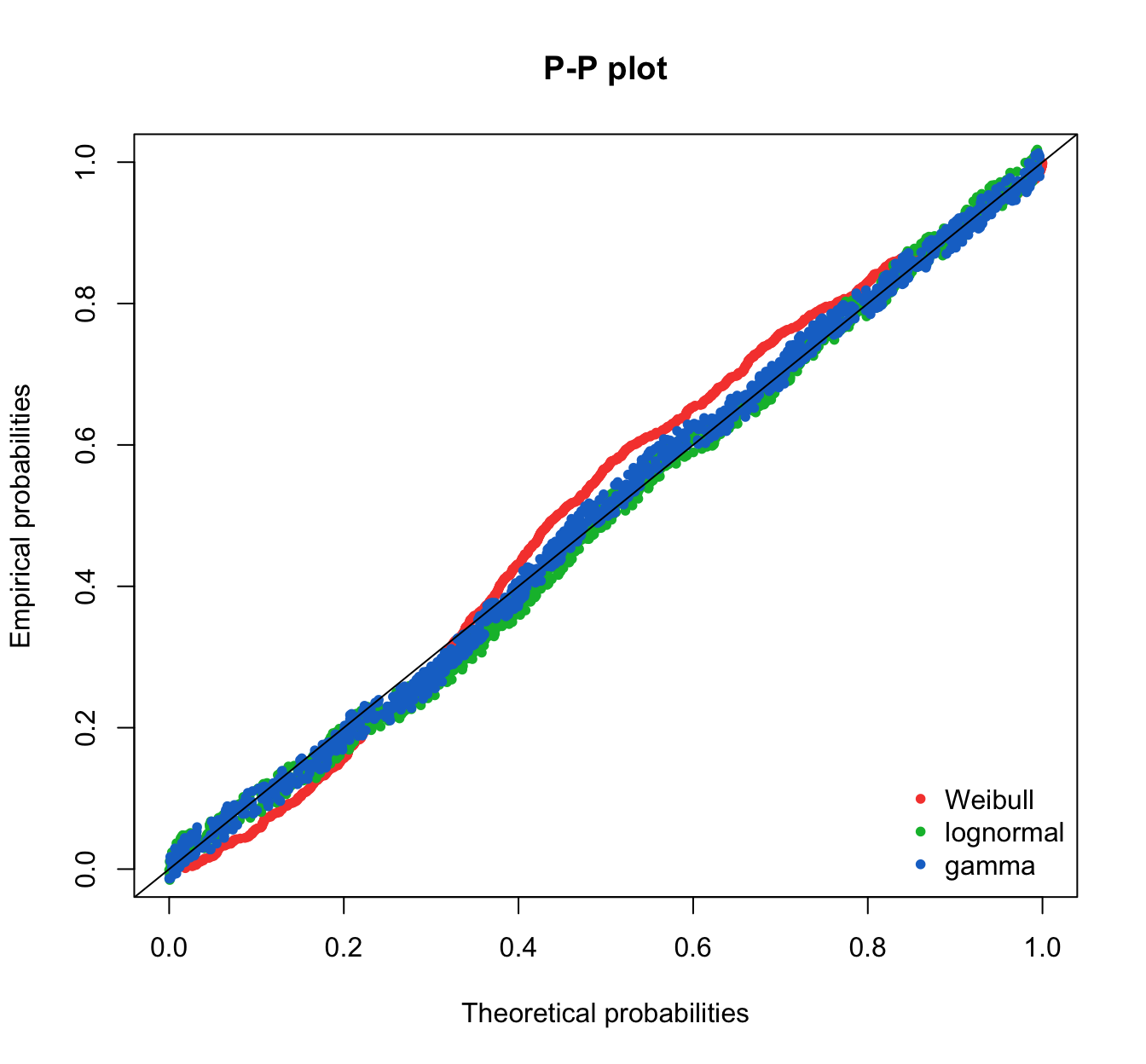
P-P plot #
To construct the P-P plot:
- order the observed data from smallest to largest:
\(x_{(1)},x_{(2)},...,x_{(n)}\). - calculate the theoretical CDF at each of the observed data points:
\(G\left( x_{(i)};\widehat{\mathbf{\theta }}\right)\). - for
\(i=1,2,...,n\), plot the points\(\dfrac{i-0.5}{n}\)against\(G\left(x_{(i)};\widehat{\mathbf{\theta }}\right)\).
Note that using \(\dfrac{i-0.5}{n}\) is Hazen’s rule, as recommended by Blom (1959).
see also the following video on YouTube:
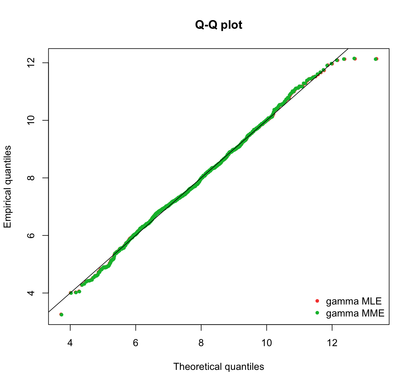
Q-Q plot #
To construct the Q-Q plot:
- order the observed data from smallest to largest:
\(x_{(1)},x_{(2)},...,x_{(n)}\). - for
\(i=1,2,...,n\), calculate the theoretical quantiles:\(G^{-1}\left(\dfrac{i-0.5}{n};\widehat{\mathbf{\theta }}\right)\). - for
\(i=1,2,...,n\), plot the points\(x_{(i)}\)against\(G^{-1}\left(\dfrac{i-0.5}{n};\widehat{\mathbf{\theta }}\right)\).
These constructions hold only for the case where you have no censoring/truncation.
see also the following video on YouTube:
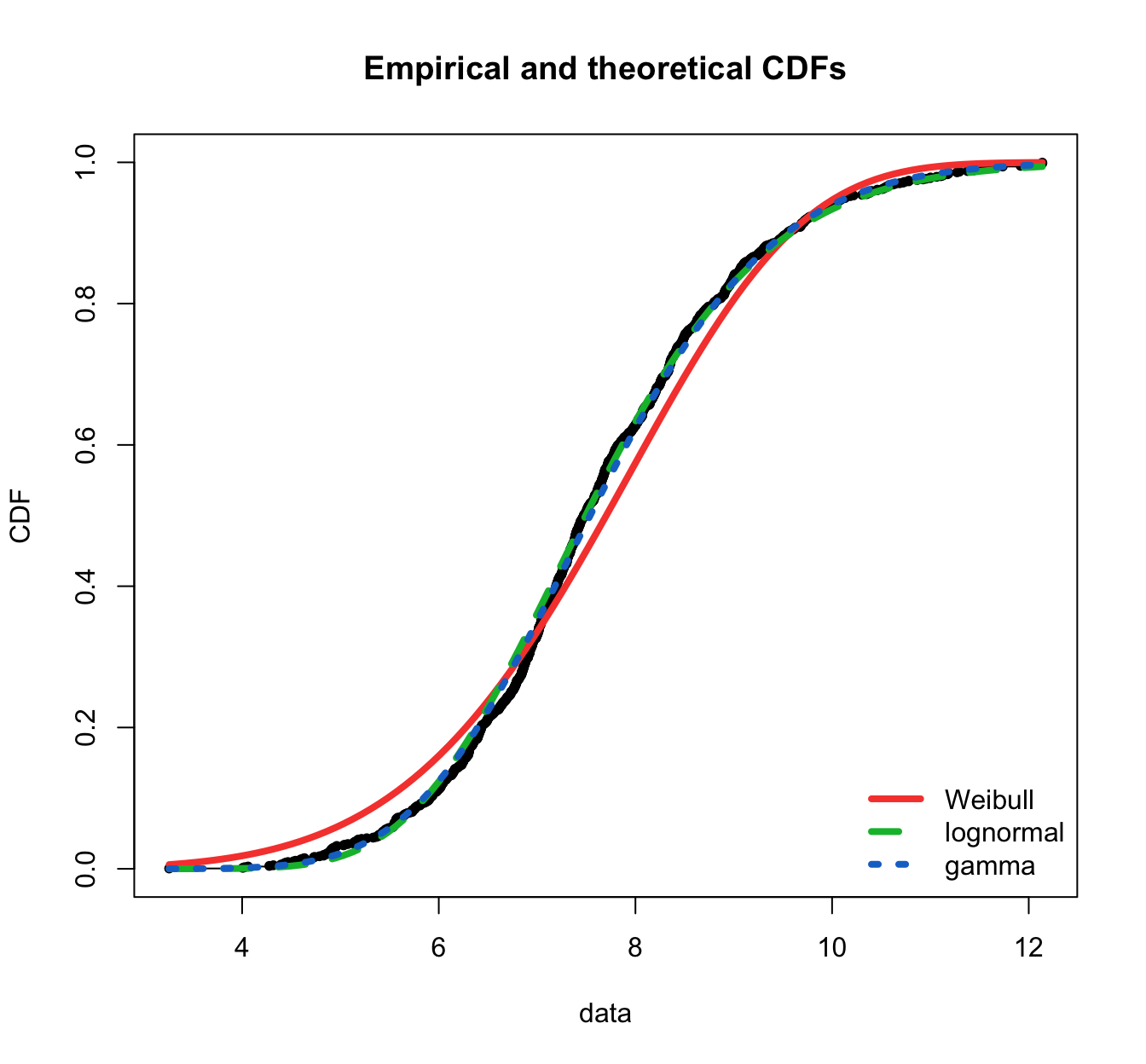
SUVA GOF graphs #
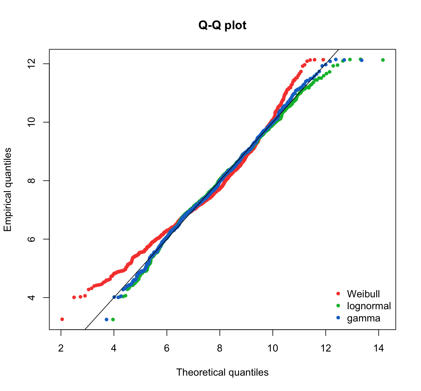
plot.legend <- c("Weibull", "lognormal", "gamma")
fitdistrplus::denscomp(list(fit.weibull.mle, fit.lnorm.mle, fit.gamma.mle),
  legendtext = plot.legend, fitlwd = 3)
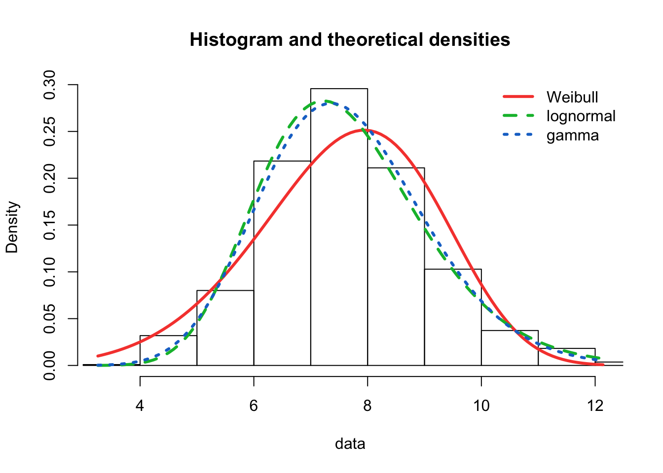
fitdistrplus::cdfcomp(list(fit.weibull.mle, fit.lnorm.mle, fit.gamma.mle),
  legendtext = plot.legend, fitlwd = 4, datapch = 20)
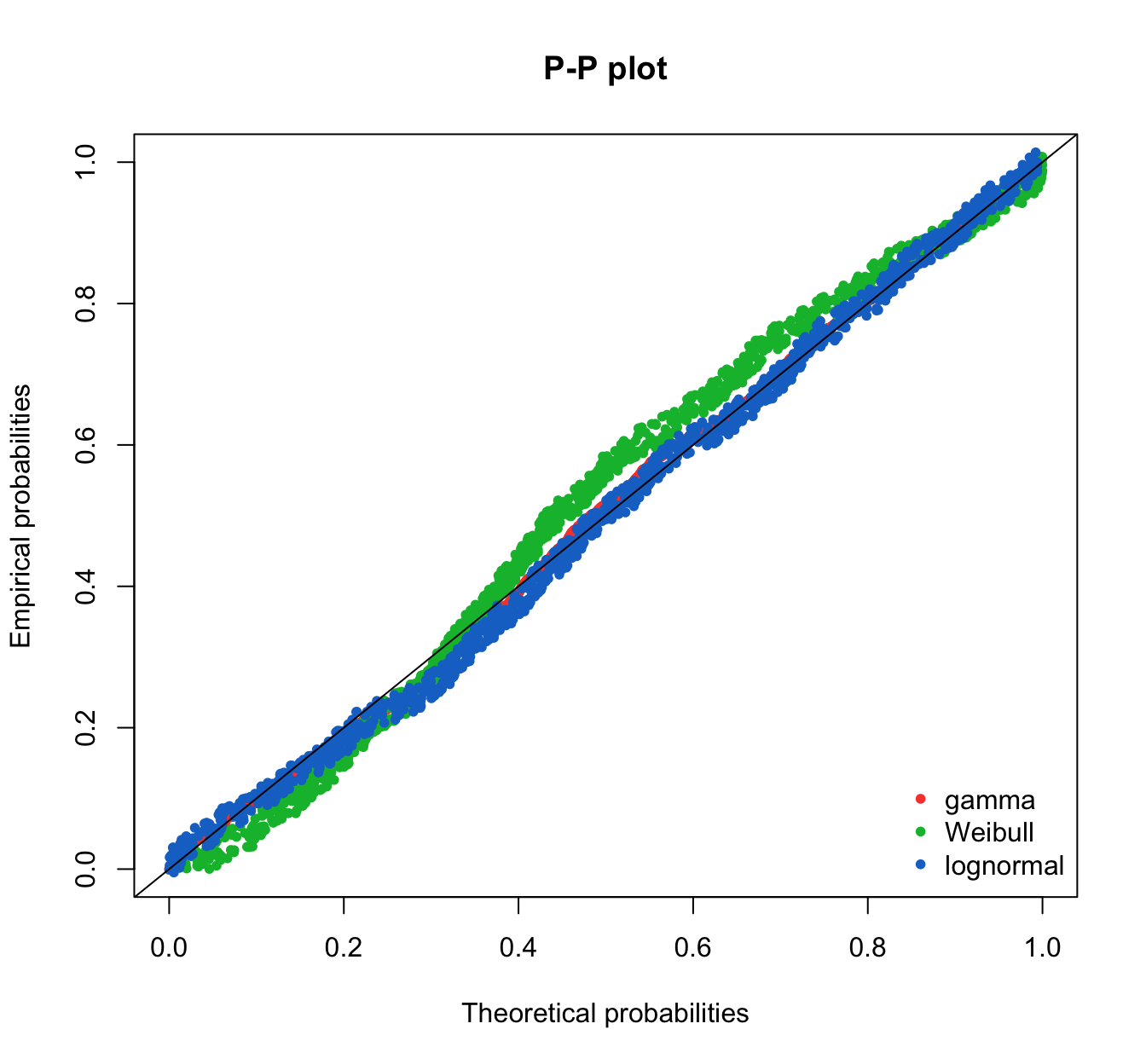
fitdistrplus::ppcomp(list(fit.weibull.mle, fit.lnorm.mle, fit.gamma.mle),
  legendtext = plot.legend, fitpch = 20)
fitdistrplus::ppcomp(list(fit.gamma.mle, fit.weibull.mle, fit.lnorm.mle),
  legendtext = c("gamma", "Weibull", "lognormal"), fitpch = 20)  #the order matters
fitdistrplus::qqcomp(list(fit.weibull.mle, fit.lnorm.mle, fit.gamma.mle),
  legendtext = plot.legend, fitpch = 20)
Hypothesis tests #
We will test the null
\(H_{0}:\)data came from population with the specified model, against\(H_{a}:\)the data did not come from such a population.
Some commonly used tests, and their test statistics:
- Kolmogorov-Smirnoff:
\(K.S.=\underset{y}{\sup }\left\vert \widehat{G} \left( y\right) -G\left( y;\widehat{\mathbf{\theta }}\right)\right\vert\) - Anderson-Darling:
\(A.D.=n \int \frac{\left[ \widehat{G}\left( y\right)-G\left( y;\widehat{\mathbf{\theta }}\right) \right] ^{2}}{G\left(y; \widehat{\mathbf{\theta }}\right) \left[ 1-G\left(y;\widehat{\mathbf{\theta }}\right) \right] } d G(y)\) \(\chi ^{2}\)goodness-of-fit:\(\chi^{2}=\sum_{j}\frac{\left(\text{observed}-\text{expected}\right) ^{2}}{\text{expected}}\)
Computational formulas for those tests are available in Delignette-Muller and Dutang (2015).
Kolmogorov-Smirnoff test #
$$K.S.=\underset{y}{\sup }\left\vert \widehat{G} \left( y\right) -G\left( y;\widehat{\mathbf{\theta }}\right) \right\vert,$$
where
\(\widehat{G}\left( y\right)\)is the empirical distribution\(G\left( y;\theta \right)\)is the assumed theoretical distribution in the null hypothesis\(G\left( y;\theta \right)\)is assumed to be (must be) continuous\(\hat{\theta}\)is the maximum likelihood estimate for\(\theta\)under the null hypothesis
Note:
- There are tables for the critical values. There are several variations of these tables in the literature that use somewhat different scalings for the K-S test statistic and critical regions.
- The test (obviously) does not work for grouped data.
Anderson-Darling test #
$$A.D.=n\int \frac{\left[ \widehat{G}\left( y\right)-G\left( y;\widehat{\mathbf{\theta }}\right) \right] ^{2}}{G\left(y; \widehat{\mathbf{\theta }}\right) \left[ 1-G\left(y;\widehat{\mathbf{\theta }}\right) \right] } d G(y),$$
where \(n\) is the sample size.
Note:
- The critical values for the Anderson-Darling test are dependent on the specific distribution that is being tested. There are tabulated values and formulas for a few specific distributions.
- The theoretical distribution is assumed to be (must be) continuous.
- The test does not work for grouped data.
\(\chi ^{2}\) goodness-of-fit test
#
Procedure:
- Break down the whole range into
\(k\)subintervals:\(c_0<c_1<\cdots<c_k=\infty\) \(\chi ^{2}\)goodness-of-fit test:\(\chi ^{2}=\sum_{j}^k\frac{(E_j-O_j)^{2}}{E_j}\)- Let
\(\hat{p_j}=G(c_j;\hat{\theta})-G(c_{j-1};\hat{\theta})\). Then, the number of expected observations in the interval\((c_{j-1},c_j]\)assuming that the hypothesized model is true:$$E_j=n\hat{p}_j \quad \text{(Here, } n \text{ is the sample size)}$$ - Let
\({p_j}=\hat{G}(c_j)-\hat{G}(c_{j-1})\). Then, the number of observations in the interval\((c_{j-1},c_j]\): $$ O_j=n{p}_j$$
The statistic has chi-square distribution with the degree of freedom
equal to: \(k-1- \alert{\text{number of parameters estimated}}\)
How these tests are used #
- Besides testing whether data came from specified model or not, generally we would prefer models with:
- lowest K-S test statistic
- lowest A-D test statistic
- lowest
\(\chi ^{2}\)goodness-of-fit test statistic (or equivalently highest\(p\)-value) - highest value of the likelihood function at the maximum
- Perform formal statistical test, or use as `horse race’
Comparison #
- K-S and A-D tests are quite similar - both look at the difference
between the empirical and model distribution functions.
- K-S in absolute value, A-D in squared difference.
- But A-D is weighted average, with more emphasis on good fit in the tails than in the middle; K-S puts no such emphasis.
- For K-S and A-D tests, no adjustments are made to account for increase in the number of parameters, nor sample size. Result: more complex models often will fare better on these tests.
- The
\(\chi ^{2}\)test adjusts the degrees of freedom for increases in the number of parameters, but is easily manipulated as the choice of brackets is arbitrary.
Information criteria #
- Information criteria penalise the log likelihood with a function that depends on the number of parameters.
- Akaike Information Criterion (AIC):
$$\text{AIC}^{(i)}=-2\ell^{(i)}_\mathbf{Y}+2d^{(i)},$$where\(d^{(i)}\)denotes the number of estimated parameters in the density\(g_i\)that is considered, and where\(\ell^{(i)}_\mathbf{Y}\)is the maximum log likelihood that can be achieved with that density. - Bayesian Information Criterion (BIC)
$$\text{BIC}^{(i)}=-2\ell^{(i)}_\mathbf{Y}+\log (n) d^{(i)}.$$This is\(-2\text{SBC}\), where SBC is Schwarz Bayesian Criterion.
- Note that these can sometimes be presented in inverse sign. Here, because the penalty is added, it is obvious that smaller values of the IC are preferred.
SUVA GOF stats #
GOF hypothesis test statistics #
For MLE:
gofstat(list(fit.weibull.mle, fit.lnorm.mle, fit.gamma.mle),
  fitnames = plot.legend)
## Goodness-of-fit statistics
##                                  Weibull  lognormal      gamma
## Kolmogorov-Smirnov statistic  0.07105097 0.04276791 0.03376236
## Cramer-von Mises statistic    1.74049707 0.26568341 0.19438834
## Anderson-Darling statistic   10.69572021 1.70209314 1.10385675
##
## Goodness-of-fit criteria
##                                 Weibull lognormal    gamma
## Akaike's Information Criterion 4010.519  3920.717 3907.636
## Bayesian Information Criterion 4020.524  3930.722 3917.641
For MME:
gofstat(list(fit.weibull.mme, fit.lnorm.mme, fit.gamma.mme),
  fitnames = plot.legend)
## Goodness-of-fit statistics
##                                  Weibull lognormal     gamma
## Kolmogorov-Smirnov statistic  0.08023228 0.0374087 0.0327241
## Cramer-von Mises statistic    1.66608962 0.1869752 0.1823197
## Anderson-Darling statistic   10.53097690 1.4369047 1.0539353
##
## Goodness-of-fit criteria
##                                 Weibull lognormal    gamma
## Akaike's Information Criterion 4044.239  3922.121 3907.677
## Bayesian Information Criterion 4054.243  3932.125 3917.681
Note that when fitting discrete distributions, the chi-squared statistic is computed by the gofstat function (see Delignette-Muller and Dutang (2015) for details).
GOF hypothesis test results #
R can also provide the results from the GOF hypothesis tests. For instance:
gammagof <- gofstat(list(fit.gamma.mle, fit.lnorm.mle), fitnames = c("gamma MLE",
  "lognormal MLE"), chisqbreaks = c(10:20/2))
gammagof$chisqpvalue
##     gamma MLE lognormal MLE
##  1.374256e-03  1.690633e-05
gammagof$adtest
##      gamma MLE  lognormal MLE
##     "rejected" "not computed"
gammagof$kstest
##      gamma MLE  lognormal MLE
## "not rejected"     "rejected"
gammagof$chisqtable
##        obscounts theo gamma MLE theo lognormal MLE
## <= 5          36       23.96251           19.19169
## <= 5.5        28       39.64865           39.53512
## <= 6          60       72.77895           76.73318
## <= 6.5       110      109.47716          116.38286
## <= 7         130      139.03193          145.08202
## <= 7.5       191      152.62949          154.45787
## <= 8         134      147.62688          144.65495
## <= 8.5       141      127.77796          121.96771
## <= 9          91      100.25469           94.30131
## <= 9.5        62       72.07629           67.84850
## <= 10         51       47.91524           45.97086
## > 10          65       65.82026           72.87394
GOF graphical comparisons #
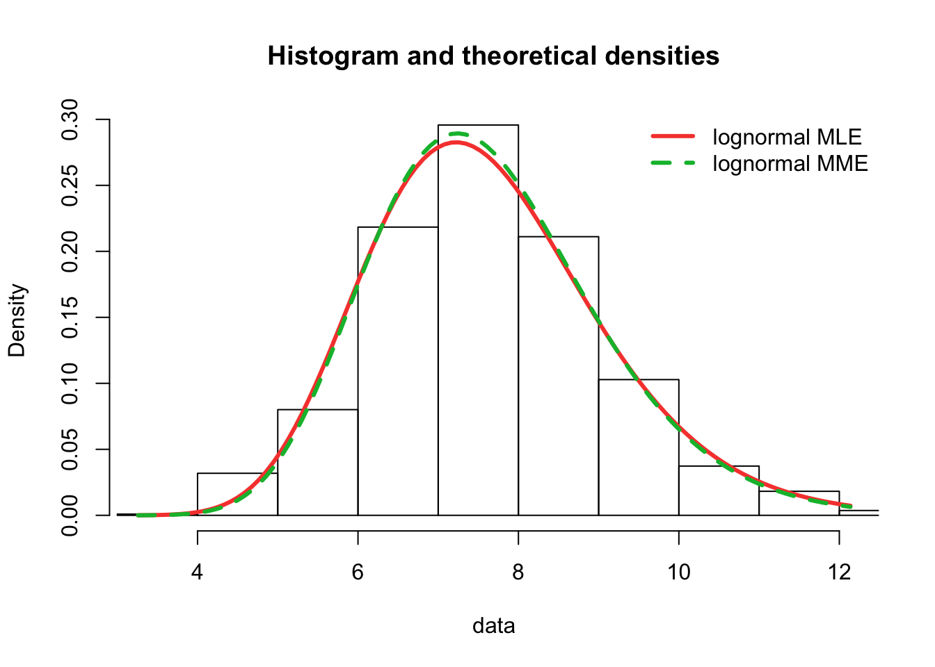
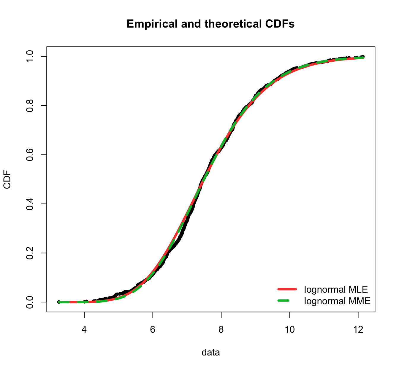
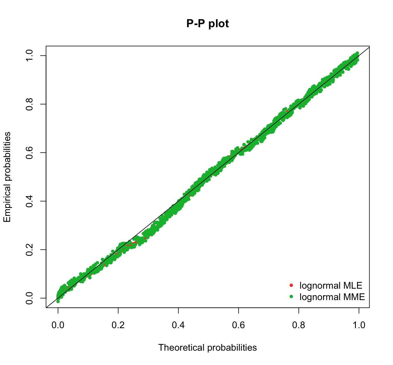
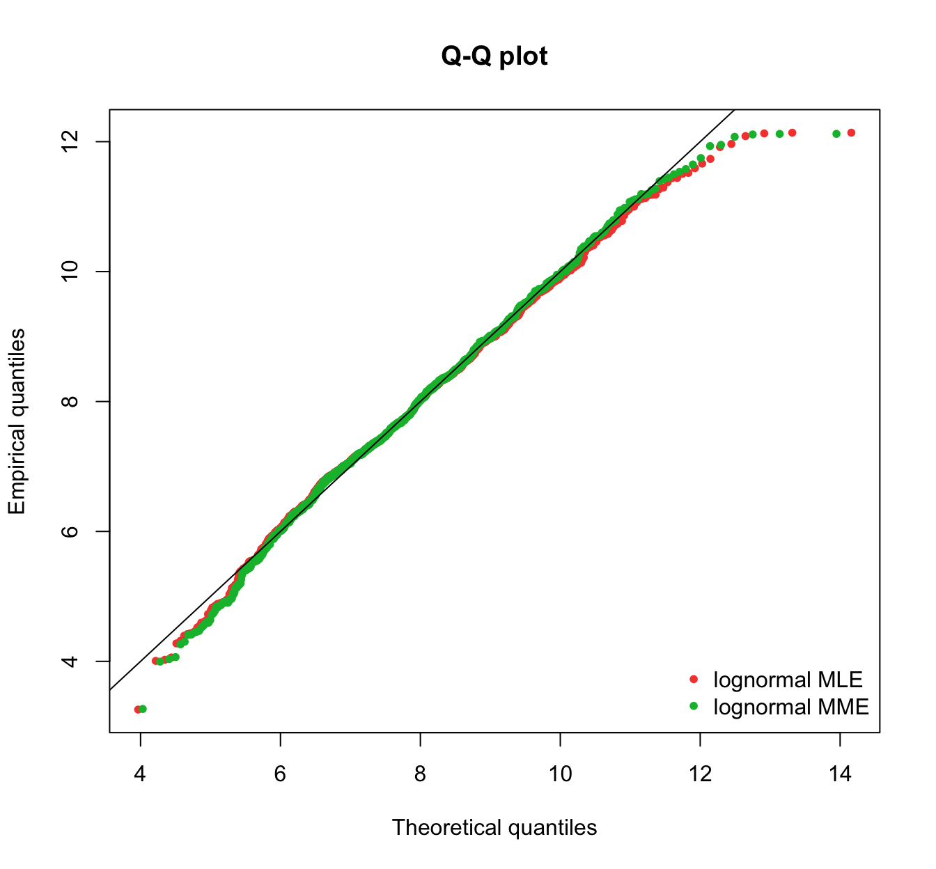
plot.legend <- c("lognormal MLE", "lognormal MME")
fitdistrplus::denscomp(list(fit.lnorm.mle, fit.lnorm.mme), legendtext = plot.legend,
  fitlwd = 3)
fitdistrplus::cdfcomp(list(fit.lnorm.mle, fit.lnorm.mme), legendtext = plot.legend,
  fitlwd = 4, datapch = 20)
fitdistrplus::ppcomp(list(fit.lnorm.mle, fit.lnorm.mme), legendtext = plot.legend,
  fitpch = 20)
fitdistrplus::qqcomp(list(fit.lnorm.mle, fit.lnorm.mme), legendtext = plot.legend,
  fitpch = 20)
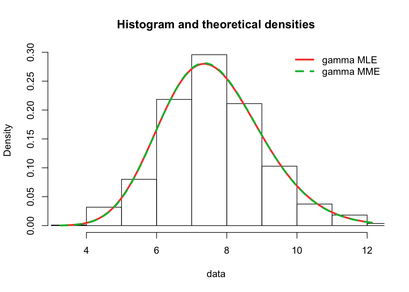
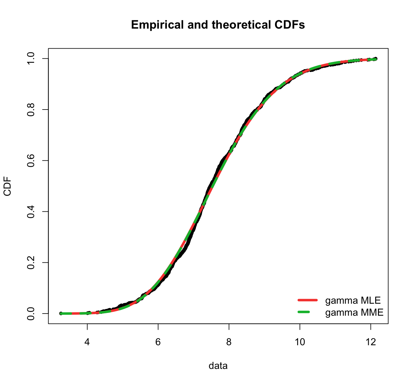
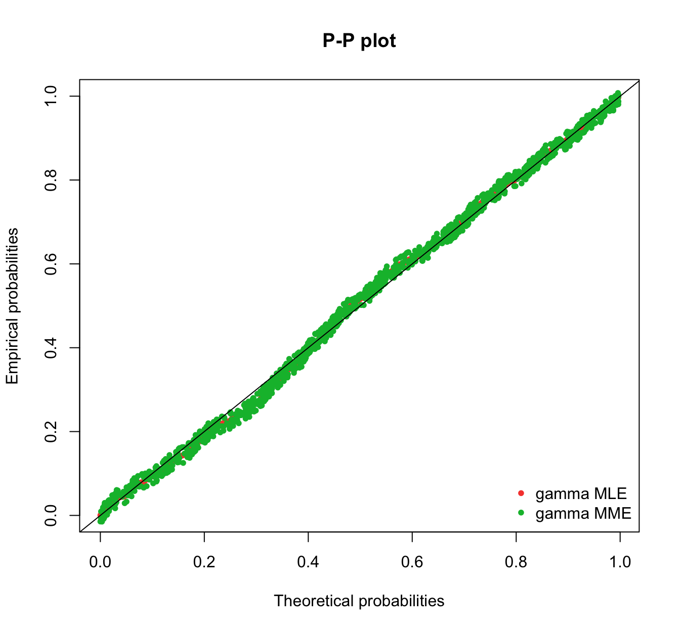
plot.legend <- c("gamma MLE", "gamma MME")
fitdistrplus::denscomp(list(fit.gamma.mle, fit.gamma.mme), legendtext = plot.legend,
  fitlwd = 3)
fitdistrplus::cdfcomp(list(fit.gamma.mle, fit.gamma.mme), legendtext = plot.legend,
  fitlwd = 4, datapch = 20)
fitdistrplus::ppcomp(list(fit.gamma.mle, fit.gamma.mme), legendtext = plot.legend,
  fitpch = 20)
fitdistrplus::qqcomp(list(fit.gamma.mle, fit.gamma.mme), legendtext = plot.legend,
  fitpch = 20)
\(\adv\) Other advanced topics
#
\(\adv\) Alternative methods for estimation
#
\(\adv\) Maximum Goodness Estimation (MGE)
#
- This is one form of “minimum distance estimation”, whereby parameters are chosen such that a distance (between empirical and theoretical) is minimised
- Here we focus on the GOF tests
AD,CvM, andKS - This can be readily chosen in R using
fitdist, withmethod="mge"and wheregof=one ofAD,CvM, orKS.
With the SUVA data:
fit.gamma.mge.ad <- fitdist(log(SUVA$dailyallow[SUVA$dailyallow >
  0]), "gamma", method = "mge", gof = "AD")
fit.gamma.mge.ks <- fitdist(log(SUVA$dailyallow[SUVA$dailyallow >
  0]), "gamma", method = "mge", gof = "KS")
gof.mge.legend <- c("gamma MLE", "gamma MGE AD", "gamma MGE KS")
gofstat(list(fit.gamma.mle, fit.gamma.mge.ad, fit.gamma.mge.ks),
  fitnames = gof.mge.legend)
## Goodness-of-fit statistics
##                               gamma MLE gamma MGE AD gamma MGE KS
## Kolmogorov-Smirnov statistic 0.03376236   0.02841676    0.0208791
## Cramer-von Mises statistic   0.19438834   0.14533386    0.1444858
## Anderson-Darling statistic   1.10385675   0.96063188    1.6991376
##
## Goodness-of-fit criteria
##                                gamma MLE gamma MGE AD gamma MGE KS
## Akaike's Information Criterion  3907.636     3908.736     3919.475
## Bayesian Information Criterion  3917.641     3918.740     3929.480
denscomp(list(fit.gamma.mle, fit.gamma.mge.ad, fit.gamma.mge.ks),
  legendtext = gof.mge.legend, fitlwd = 3)
cdfcomp(list(fit.gamma.mle, fit.gamma.mge.ad, fit.gamma.mge.ks),
  legendtext = gof.mge.legend, fitlwd = 4, datapch = 20)
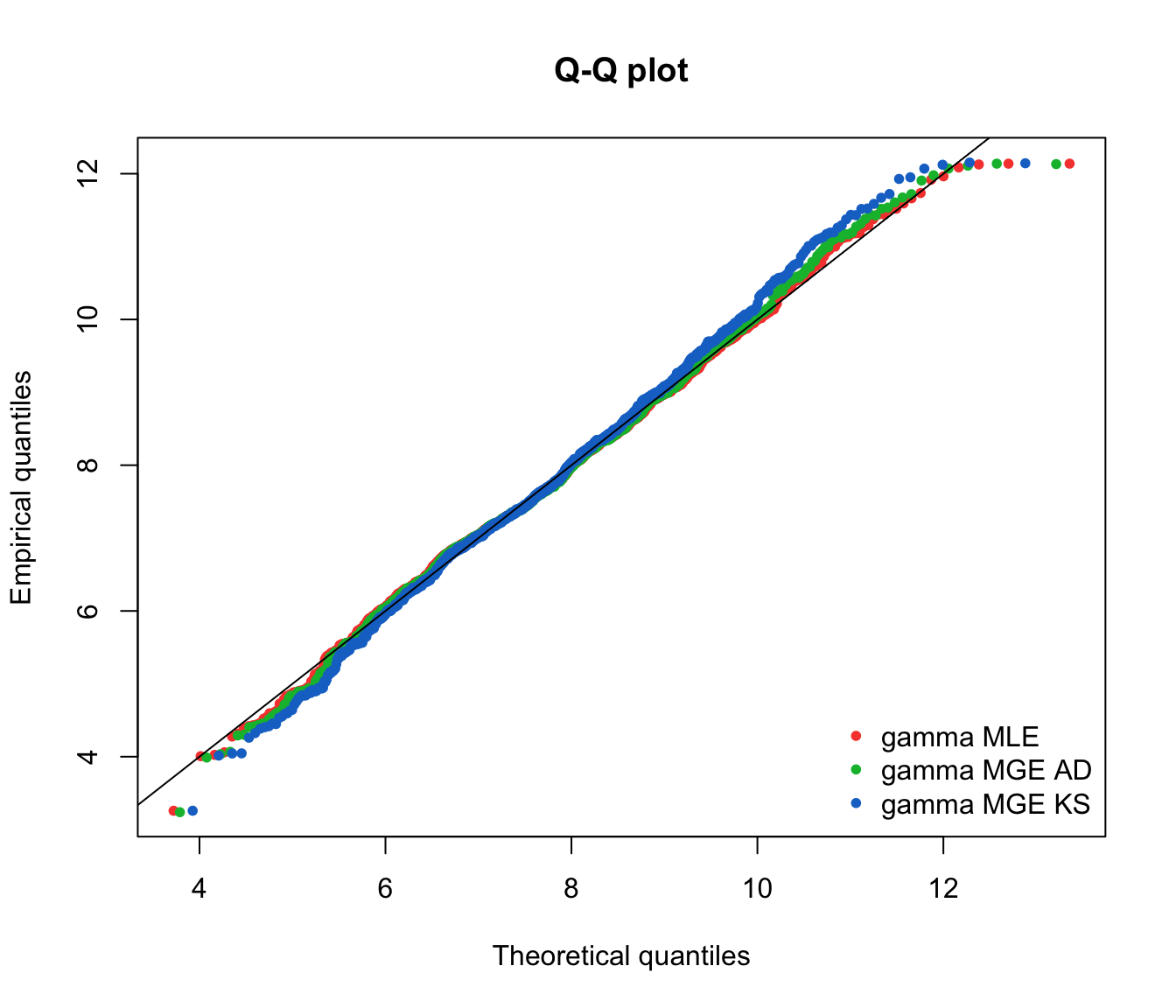
ppcomp(list(fit.gamma.mle, fit.gamma.mge.ad, fit.gamma.mge.ks),
  legendtext = gof.mge.legend, fitpch = 20)
qqcomp(list(fit.gamma.mle, fit.gamma.mge.ad, fit.gamma.mge.ks),
  legendtext = gof.mge.legend, fitpch = 20)
\(\adv\) AD based parameter estimation
#
- Recall the Anderson-Darling test statistic, which focused on the tails.
- What if we wanted to generalise the idea of AD to left tail or right tail only, or put even more weight on either of those tails?
- The AD test considers a weighted “sum” (integral) of the squared difference between empirical and theoretical cdf’s
- In its original formulation, the weight is of the form
$$ w_i= \frac{1}{G(y) [1-G(y)]},$$
which goes to infinity when
\(y\rightarrow 0\)or\(y\rightarrow \infty\). - There are 5 alternatives in
fitdistrplus.
ADR: Right-tail AD, where$$w_i = \frac{1}{1-G(y)};$$ADL: Left-tail AD, where$$w_i = \frac{1}{G(y)};$$ADR2: Right-tail AD, 2nd order, where$$w_i = \frac{1}{[1-G(y)]^2};$$ADL2: Left-tail AD, 2nd order, where$$w_i = \frac{1}{[G(y)]^2};$$AD2: AD, 2nd order. Here,Rwill minimiseADR2+ADL2.
With the SUVA data:
fit.gamma.mge.adr <- fitdist(log(SUVA$dailyallow[SUVA$dailyallow >
0]), "gamma", method = "mge", gof = "ADR")
fit.gamma.mge.adr2 <- fitdist(log(SUVA$dailyallow[SUVA$dailyallow >
0]), "gamma", method = "mge", gof = "AD2R")
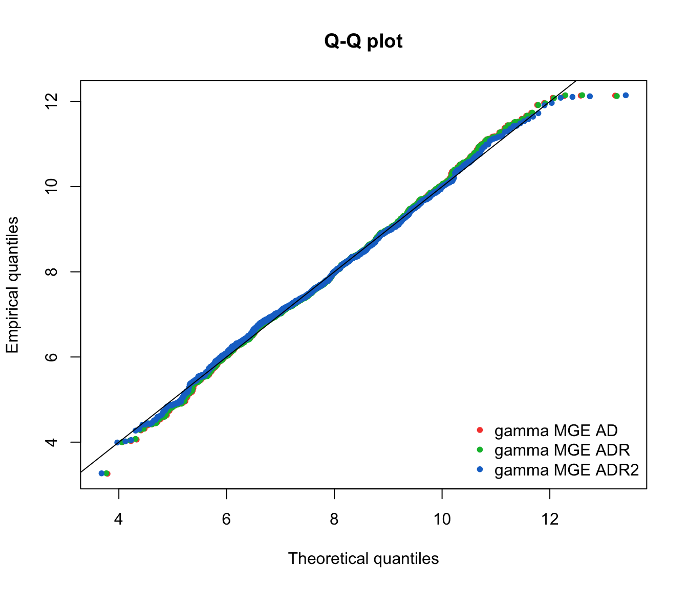
gof.mge.legend2 <- c("gamma MGE AD", "gamma MGE ADR", "gamma MGE ADR2")
gofstat(list(fit.gamma.mge.ad, fit.gamma.mge.adr, fit.gamma.mge.adr2),
  fitnames = gof.mge.legend2)
## Goodness-of-fit statistics
##                              gamma MGE AD gamma MGE ADR
## Kolmogorov-Smirnov statistic   0.02841676     0.0309970
## Cramer-von Mises statistic     0.14533386     0.1553754
## Anderson-Darling statistic     0.96063188     0.9799768
##                              gamma MGE ADR2
## Kolmogorov-Smirnov statistic     0.03980158
## Cramer-von Mises statistic       0.24760685
## Anderson-Darling statistic       1.38154307
##
## Goodness-of-fit criteria
##                                gamma MGE AD gamma MGE ADR
## Akaike's Information Criterion     3908.736      3908.223
## Bayesian Information Criterion     3918.740      3918.228
##                                gamma MGE ADR2
## Akaike's Information Criterion       3908.049
## Bayesian Information Criterion       3918.054
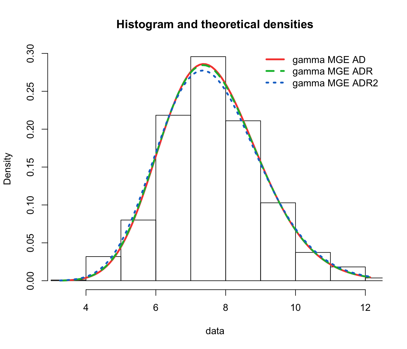
denscomp(list(fit.gamma.mge.ad, fit.gamma.mge.adr, fit.gamma.mge.adr2),
  legendtext = gof.mge.legend2, fitlwd = 3)
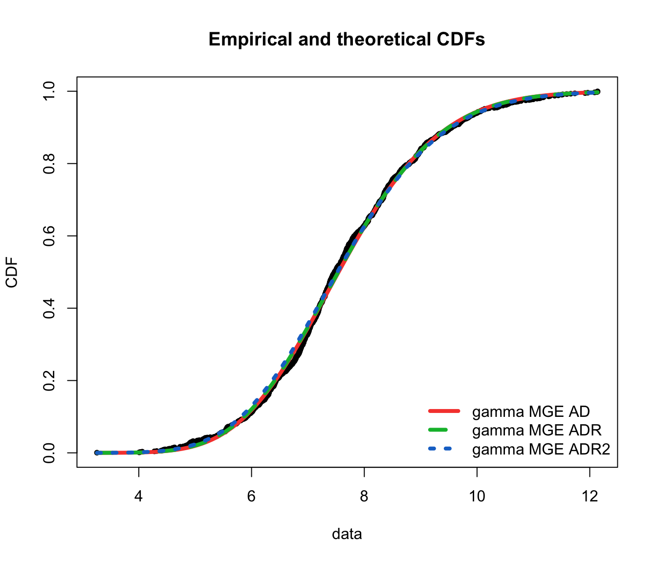
cdfcomp(list(fit.gamma.mge.ad, fit.gamma.mge.adr, fit.gamma.mge.adr2),
  legendtext = gof.mge.legend2, fitlwd = 4, datapch = 20)
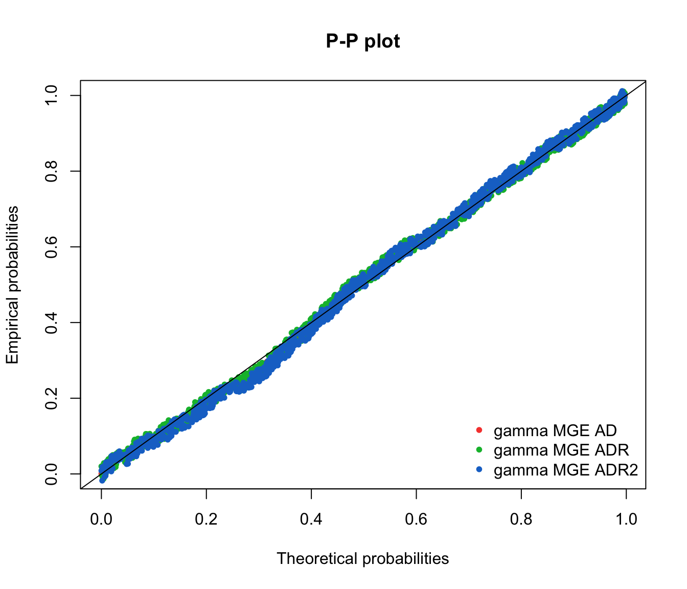
ppcomp(list(fit.gamma.mge.ad, fit.gamma.mge.adr, fit.gamma.mge.adr2),
  legendtext = gof.mge.legend2, fitpch = 20)
qqcomp(list(fit.gamma.mge.ad, fit.gamma.mge.adr, fit.gamma.mge.adr2),
  legendtext = gof.mge.legend2, fitpch = 20)
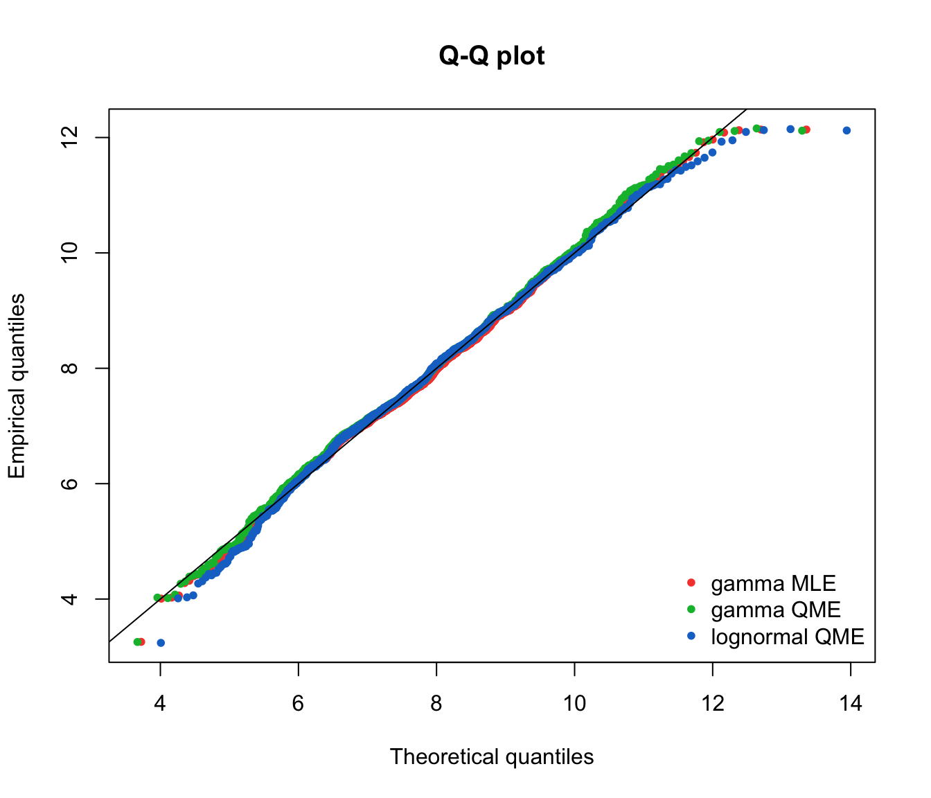
\(\adv\) Quantile matching
#
- Quantile matching is easily implemented in R:
- set
method="qme"in the call tofitdist; - and add an argument
probsdefining the probabilities for which the quantile matching is performed.
- set
- The number of quantiles to match must be the same as the number of parameters to estimate.
- The quantile matching is carried out numerically, by minimising the sum of squared differences between observed and theoretical quantiles.
For example:
fit.gamma.qme <- fitdist(log(SUVA$dailyallow[SUVA$dailyallow >
0]), "gamma", method = "qme", probs = c(0.5, 0.75))
fit.lnorm.qme <- fitdist(log(SUVA$dailyallow[SUVA$dailyallow >
0]), "lnorm", method = "qme", probs = c(0.5, 0.75))
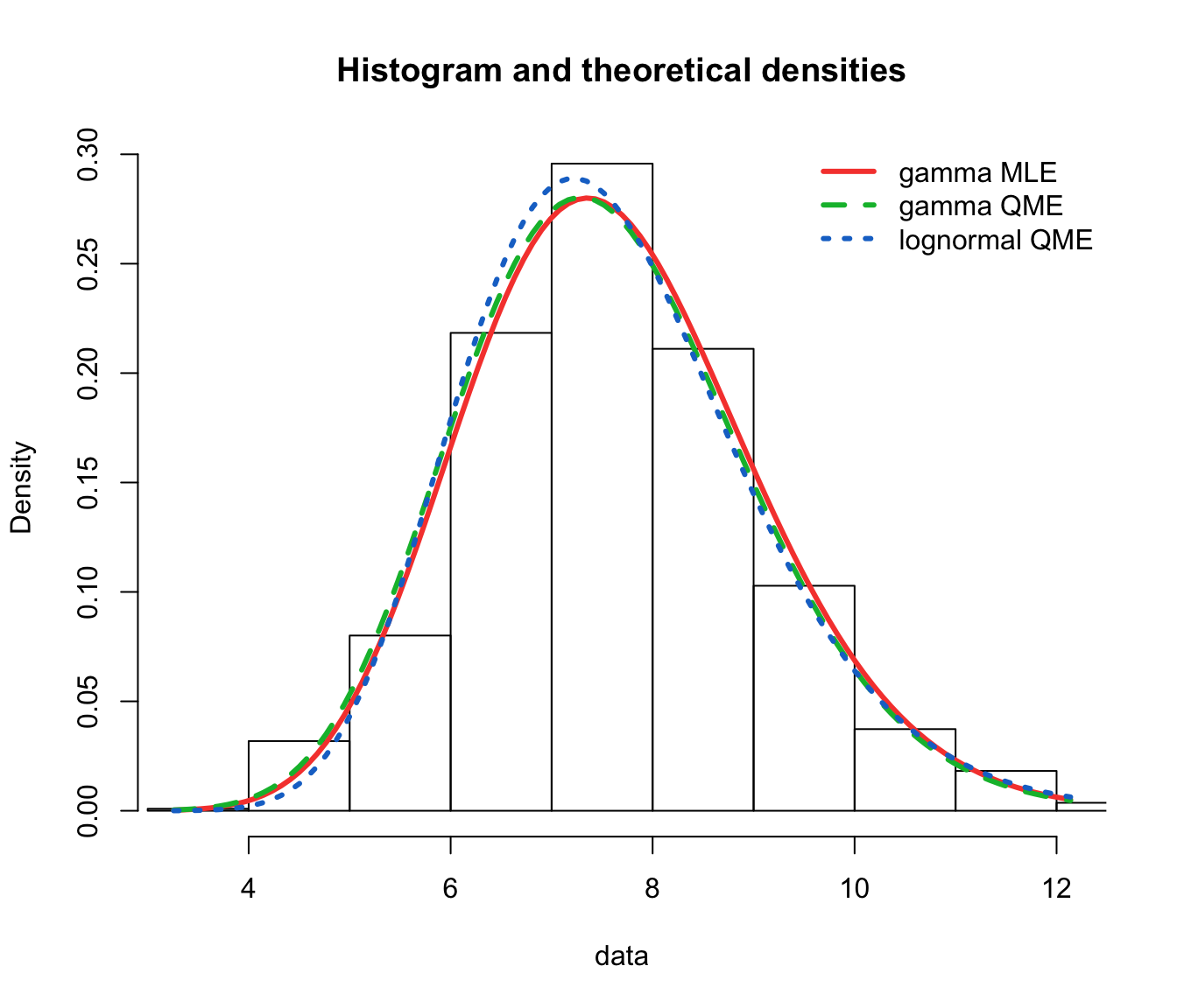
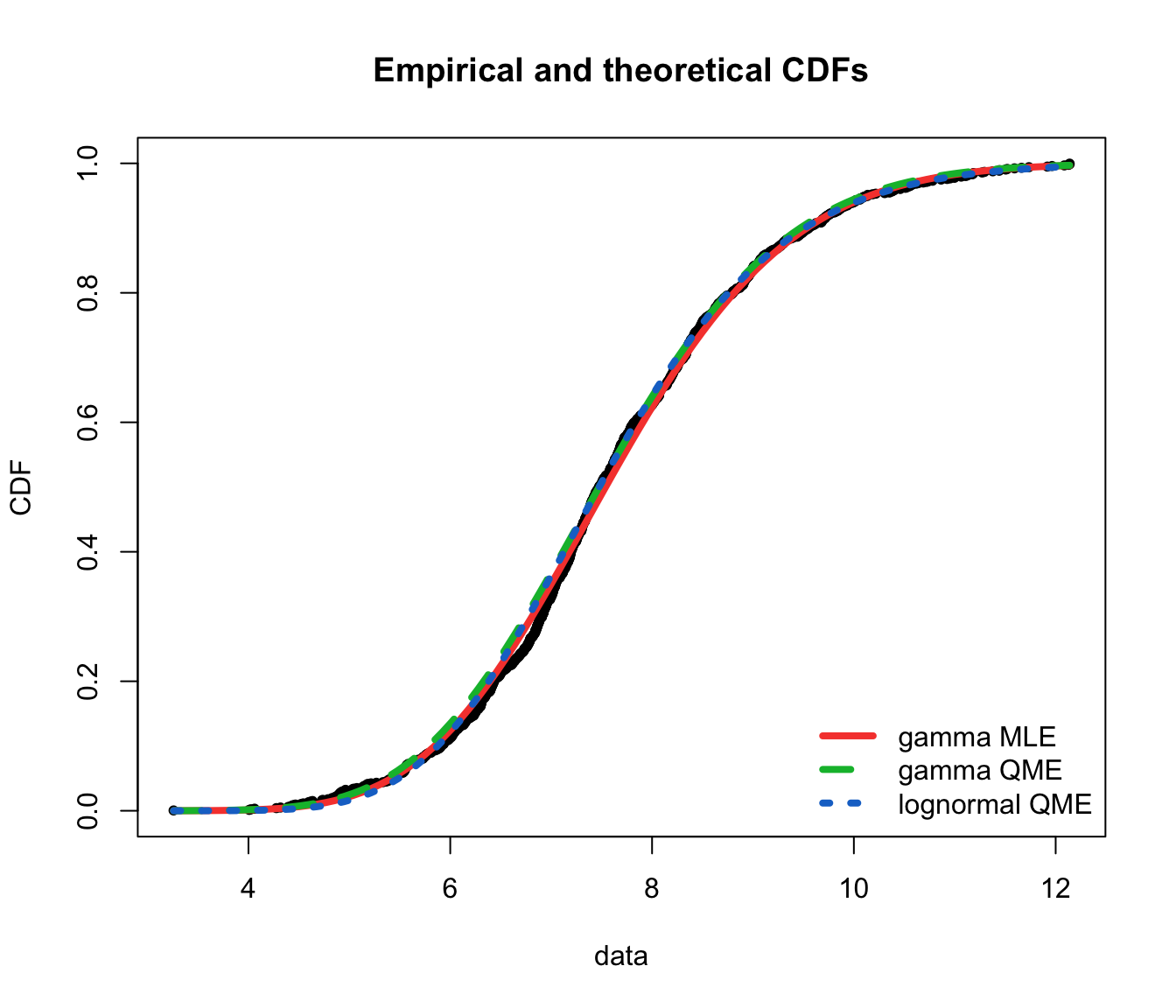
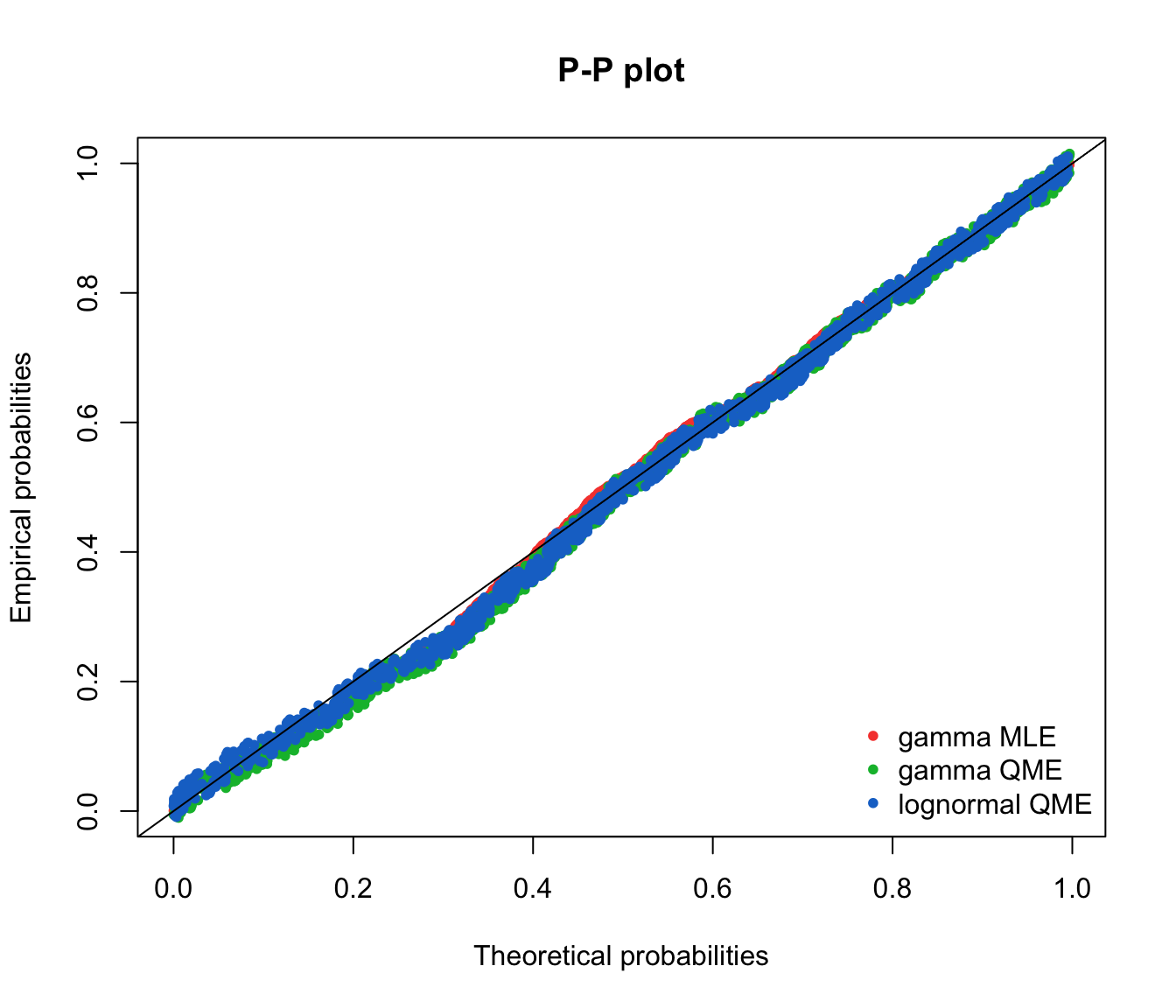
gof.qme.legend <- c("gamma MLE", "gamma QME", "lognormal QME")
denscomp(list(fit.gamma.mle, fit.gamma.qme, fit.lnorm.qme), legendtext = gof.qme.legend,
  fitlwd = 3)
cdfcomp(list(fit.gamma.mle, fit.gamma.qme, fit.lnorm.qme), legendtext = gof.qme.legend,
  fitlwd = 4, datapch = 20)
ppcomp(list(fit.gamma.mle, fit.gamma.qme, fit.lnorm.qme), legendtext = gof.qme.legend,
  fitpch = 20)
qqcomp(list(fit.gamma.mle, fit.gamma.qme, fit.lnorm.qme), legendtext = gof.qme.legend,
  fitpch = 20)
\(\adv\) Zero-inflated severity model \(X=IB\)
#
In this approach \(X=IB\), where
\(I\)is an indicator of claim with$$\Pr\left[ I=1\right] =q\text{ and }\Pr\left[ I=0\right] =1-q$$\(B\)is the {claim amount given\(I=1\)} (given a claim occurs).
This allows us to avoid a large probability mass at 0 for rare losses.
- Note that this is a good approach for modifying continuous distributions, which are generally used for severity.
- In the case of discrete distributions—usually used for frequency, modifications of the usual distributions (in the form of “zero-truncated” or “zero-modified”) are well known, and readily available in the package
actuar. This is discussed in Module 2. - In practice a frequency and severity model would be chosen at the same time, and the way zero claims are dealt with should be determined in a consistent way, e.g.:
- “frequency” models strictly positive claims, and “severity” is a strictly positive continuous distribution;
- “frequency” models insurable events (which may lead to claims of 0), and “severity” includes a mass at 0 (such as in this section);
- etc…
\(\adv\) Resulting distribution
#
As a consequence,
$$\begin{array}{rcl} \Pr\left[ X\leq x \right] &=&\Pr\left[ X\leq x | I=0\right]\Pr[I=0]\\&&+\Pr\left[ X\leq x | I=1\right]\Pr[I=1] \\ &=&1-q+q\Pr\left[ B\leq x \right] \end{array}$$
and
$$\begin{array}{rcl} M_X(t)&=&E[e^{tX}|I=0]\Pr[I=0]\\ &&+E[e^{tX}|I=1]\Pr[I=1]\\ &=&1-q+q E[e^{tB}]. \end{array}$$
\(\adv\) Mean and Variance
#
The mean can be determined using
$$E\left[ X\right] =E\left[ E\left[ X\left\vert I\right. \right]\right] =E\left[ X\left\vert I\right. =1\right] \Pr\left[ I=1\right]=qE\left( B\right),$$
after noting that \(E\left[ X\left\vert I\right. =0\right] =0\).
The variance can be determined using
$$\begin{array}{rcl} Var\left( X\right) &=&Var\left( E\left[ X\left\vert I\right.\right] \right)+E\left[ Var\left( X\left\vert I\right. \right) \right] \\ &=&\left[ E\left( B\right) \right] ^{2}Var\left( I\right)+qVar\left(B\right) \\ &=&q\left( 1-q\right) \left( E\left[ B\right] \right)^{2}+qVar\left( B\right) \end{array}$$
after noting that
$$\begin{array}{rcl} E[ X|I] &=&I \cdot E[ B],\text{ and that} \\ Var( X| I)&=&I^2 \cdot Var(B), \end{array}$$
which are both random variables (functions of \(I\)).
\(\adv\) Special case: \(X=Ib\)
#
- Fixed claim:
\(B=b\)with probability 1. - The individual claim random variable becomes
$$X=Ib=\left\{ \begin{array}{ll} b, & \text{w.p. }q \\ 0, & \text{w.p. }1-q \end{array} \right. \text{.}$$ - Mean:
\(E\left[ X\right] =bq\) - Variance:
\(Var\left( X\right) =b^{2}Var\left( I\right)=b^{2}q\left( 1-q\right)\)
This is nothing more than a scaled Bernoulli… (and if you add them, the sum becomes a scaled Binomial)
\(\adv\) Example: Bicycle Theft (get \(B\) out of \(X\))
#
- Insurance policy against bicycle theft (insured amount is 400)
- Only half is paid if bicycle is not locked.
- Assume:
\(\Pr\left[ X=400\right] =0.05\)and\(\Pr\left[X=200\right] =0.15\). - Probability of a claim:
\(q=\Pr\left[ I=1\right] =0.20\)[law of total probability] - The pmf of
\(B\)is computed in the following way
$$\begin{array}{rcl} \Pr\left[ B=400 \right] &=&\Pr[ X=400 | I=1] = \frac{\Pr[X=400 \ \cap\ I=1]}{\Pr[I=1]}\\ &=&\frac{0.05}{0.20} = 0.25 \end{array}$$
\(\adv\) Example
#
In an insurance portfolio, there are 15 insured:
- ten of the insured persons have 0.1 probability of making a claim, and
- the other 5 have a 0.2 probability of making a claim.
All claims are independent and follow an exponential distribution with mean \(1/\lambda\). What is the mgf of the aggregate claims distribution?
Let \(X_i\) be the total amount of claims incurred from the \(i\)th person, and \(B_i\) denote the amount of claim, if there is one. Then \(X_i=I_iB_i\).
If \(q_i=\Pr(I_i=1)\) then \(q_1=\cdots=q_{10}=0.1\) and \(q_{11}=\cdots=q_{15}=0.2.\)
The mgf of \(X_i\):
$$\begin{array}{rcl} M_{X_i}(t)&=&E[e^{tX_i}|I_i=0]\Pr(I_i=0)+E[e^{tX_i}|I_i=1]\Pr(I_i=1) \\ &=&1-q_i+E[e^{tB_i}]q_i=1-q_i+\frac{\lambda}{\lambda-t}q_i \end{array}$$
Since the aggregate claims are \(S=X_1+\cdots+X_{15}\) the mgf of \(S\) is
$$\begin{array}{rcl} M_{S}(t)&=&\prod_{i=1}^{15}E[e^{tX_i}] \\ &=&\left(1-0.1+0.1\frac{\lambda}{\lambda-t}\right)^{10}\left(1-0.2+0.2\frac{\lambda}{\lambda-t}\right)^{5} \end{array}$$
Calculating within layers for claim sizes (MW 3.4) #
Usual policy transformations #
Deductible and Policy Limit #
One way to control the cost (and variability) of individual claim losses is to introduce deductibles and policy limits.
- Deductible
\(d\): the insurer starts paying claim amounts above the deductible\(d\) - Limit
\(M\): the insurer pays up to the limit\(M\).
If we denote the damage random variable by \(D\), then if a claim occurs the insurer is liable for
$$X=\min \left[ \max \left( D-d,0\right) ,M\right] \text{.}$$
Reinsurance #
Reinsurance is a risk transfer from an insurer (the direct writer) to a reinsurer:
- in other words, some of the (random) risk faced by the insurer is “transfered” to the reinsurer (that means the reinsurer will cover that risk), in exchange of a (deterministic) premium (which will obviously generally be higher than the expected value of the risk that was transferred)
- the risk that the insurer keeps is called the retention
There are different types of reinsurance:
- proportional
- quota share: the proportion is the same for all risks
- surplus: the proportion can vary from risk to risk
- nonproportional
- (individual) excess of loss: on each individual loss
\((X_i)\) - stop loss: on the aggregate loss
\((S)\)
- (individual) excess of loss: on each individual loss
- cheap (reinsurance premium is the expected value), or non cheap (reinsurance premium is loaded)
- Alternative Risk Transfers (“ART”), where usually the idea is to transfer the risk to different / deeper pockets. For instance, for transfers to the financial markets:
- Catastrophe bonds (“CAT bonds”)
- Longevity bonds
- Pandemic bonds
Proportional reinsurance #
The retained proportion \(\alpha\) defines who pays what:
- the insurer pays
\(Y=\alpha X\) - the reinsurer pays
\(Z=(1-\alpha) X\)
This is nothing else but a change of scale and we have
$$\mu_Y=\alpha \mu_X,\;\;\;\sigma^2_Y=\alpha^2\sigma^2_X,\;\;\;\gamma_Y=\gamma_X.$$
In some cases it suffices to adapt the scale parameter. Example:
- If
\(X\)is exponential with parameter\(\beta\)$$\Pr[Y\le y]=\Pr[\alpha X \le y]=\Pr[X \le y/\alpha] = 1-e^{-\beta y / \alpha}$$and thus\(Y\)is exponential with parameter\(\beta/\alpha\).
Nonproportional reinsurance #
Basic arrangements:
- the reinsurer pays the excess over a retention (excess point)
\(d\)- the insurer pays
\(Y=\min(X,d)\) - the reinsurer pays
\(Z=(X-d)_+\)\(E[(X-d)_+]\)is called stop-loss premium.
- the insurer pays
- the reinsurer limits his payments to an amount
\(M\). In that case- the insurer pays
\(Y=\min(X,d)+(X-M-d)_+\) - the reinsurer pays
\(Z=\min\left\{(X-d)_+,M\right\}\)
- the insurer pays
Example #
Consider a life insurance company with \(16,\!000\) 1-year term life insurance policies. The associated insured amounts are:
| Benefit (10000’s) | # policies |
|---|---|
| 1 | 8000 |
| 2 | 3500 |
| 3 | 2500 |
| 5 | 1500 |
| 10 | 500 |
The probability of death \((q)\) for each of the \(16,\!000\) lives is 0.02. This company has an EoL reinsurance contract with retention limit \(30,\!000\) at a cost of 0.025 per dollar of coverage.
What is the approximate probability (using CLT) that the total cost will exceed \(8,\!250,\!000\)?
The portfolio of retained business is given by
\(k\) |
retained benefit \(b_k\) (10000’s) |
# policies \(n_k\) |
|---|---|---|
| 1 | 1 | 8000 |
| 2 | 2 | 3500 |
| 3 | 3 | 4500 |
Now
$$\begin{array}{rcl} E[S]&=&\sum_{k=1}^3 n_k E[X_k]=\sum_{k=1}^3 n_k b_kq_k \\ &=& 8000\cdot1\cdot 0.02+3500\cdot2\cdot 0.02+4500\cdot3\cdot 0.02 \\ &=&570,\quad\text{ and} \\ Var[S]&=&\sum_{k=1}^3 n_k Var[X_k]=\sum_{k=1}^3 n_k b_k^2q_k(1-q_k) \\ &=& 8000\cdot1^2\cdot 0.02\cdot 0.98+3500\cdot2^2\cdot 0.02\cdot 0.98 \\ &&+4500\cdot3^2\cdot 0.02\cdot 0.98\\&=&1225 \end{array}$$
The reinsurance cost is
$$[(5-3)\cdot 1500+(10-3)\cdot 500] \cdot 0.025=162.5.$$
Thus, the desired probability becomes
$$\begin{array}{rcl} \Pr[S+162.5>825]&=&\Pr\left[\frac{S-E[S]}{\sqrt{Var(S)}}>\frac{662.5-E[S]}{\sqrt{Var(S)}}\right] \\ &\approx& \Pr\left[Z>\frac{662.5-570}{\sqrt{1225}}\right] \\ &=&\Pr[Z>2.643]=0.0041. \end{array}$$
Discussion:
- Without reinsurance, exp/var is 700/2587.20 so the associated probability of shortfall is
\(\approx \Pr[Z>2.458]\), which is higher even though it is not cheap reinsurance. - However, there is lower expected gain:
- With reinsurance the expected gain is
$$P-570-162.5=P-732.5$$ - Without reinsurance it is
$$P-700,$$which is higher.
- With reinsurance the expected gain is
\(\adv\) The actuar coverage function
#
- The package
actuarallows for direct specification of the pdf of a modified random variable after possible left-trunction and right-censoring. - Given the pdf or cdf of the original loss
\(D\),coveragereturns a function object to compute the pdf or cdf of the modified random variable after one or several of the following modifications:- ordinary deductible
\(d\); - franchise deductible
\(d\); - limit
\(u\); - coinsurance
\(\alpha\); - inflation
\(r\).
- ordinary deductible
- The
vignette on loss modeling features of
actuarprovides precise definitions, and this document summarises all the formulas.
Assume that insurance payments are
$$X = \left\{ \begin{array}{cc} D-d, & d\le D\le u \\ u-d, & D\ge u \end{array}\right.$$
with mixed distribution
$$f_X(y) = \left\{ \begin{array}{cc} 0, & x=0 \\ \frac{f_D(y+d)}{1-F_D(d)}, & 0< x < u-d \\ \frac{1-F_D(u)}{1-F_D(d)}, & x=u-d \\ 0 & x>u-d \end{array}\right.$$
as seen before. Note however that the \(u\) is expressed on the raw variable \(D\), not the payment, so that the maximum payment is \(u-d\).
If \(D\) is gamma, \(d=2\), and \(u=20\), one can get \(f_X(x)\) in R as follows:
f <- coverage(pdf = dgamma, cdf = pgamma, deductible = 2, limit = 20)
The function can be then used to fit distributions to data.
As an example we will use the previously generated data xcens. Note it needs to be shifted by \(d\) down, because what we have is the left-truncated and right-censored \(D\), not the insurance payments as per the formulation above.
fit.gamma.xcens2 <- fitdistr(xcens$left - 2, f, start = list(shape = mean(xcens$left)^2/var(xcens$left),
  rate = mean(xcens$left)/var(xcens$left)))
fit.gamma.xcens2
##      shape         rate
##   2.03990496   0.20142871
##  (0.10516140) (0.01009694)
fit.tgamma.xcens  # our previous fit with fitdist
## Fitting of the distribution ' tgamma ' on censored data by maximum likelihood
## Parameters:
##        estimate
## shape 2.0296237
## rate  0.2006534
## Fixed parameters:
##        value
## low 2.013575
c(fit.gamma.xcens2$loglik, fit.tgamma.xcens$loglik)
## [1] -5341.551 -5340.151
Note that this is using MASS::fitdistr rather than the (arguably more flexible and possibly advanced) fitdistrplus::fitdist. This approach works as well, but does not seem as precise in this particular instance.
A useful identity #
Note that
$$\min(X,c)=X-(X-c)_+$$
and thus
$$E[\min(X,c)]=E[X]-E[(X-c)_+].$$
The amount \(E[(X-c)_+]=\Pr[X>c]e(c)\)
- is commonly called “stop loss premium” with retention
\(c\). - is identical to the expected payoff of a call with strike price
\(c\), and thus results from financial mathematics can sometimes be directly used (and vice versa).
Stop loss premiums #
Let
$$E[(X-d)_+]=P_d.$$
Then we have (for positive rv’s)
$$P_d=\left\{ \begin{array}{ll}\int_d^\infty \left[1-F_X(x)\right] dx & \text{if }X\text{ is continuous} \\ \sum_d^\infty \left[1-F_X(x)\right] & \text{if }X\text{ is discrete} \end{array}\right.$$
Example #
Calculate \(P_d\) if \(X\) is Exponential with mean \(1/\beta\).
\(\adv\) Recursive formulas in the discrete case
#
First moment:
- if
\(d\)is an integer$$P_{d+1}=P_d-[1-F_X(d)]\text{ with }P_0=E[X]$$ - if
\(d\)is not an integer$$P_d=P_{\lfloor d \rfloor}-(d-\lfloor d \rfloor)[1-F_X(\lfloor d \rfloor)].$$Second moment\(P^2_d=E[(X-d)_+^2]\):$$P_{d+1}^2=P_{d}^2-2P_{d}+[1-F_X(d)]\text{ with }P_0^2=E[X^2].$$
Note that \(\lfloor x \rfloor\) is the integer part of \(x\) (e.g. \(\lfloor 2.5 \rfloor=2\)).
\(\adv\) Numerical example
#
For the distribution \(F_{1+2+3}\) derived in Module 2 we have \(E[S]=4=128/32\) and \(E[S^2]=19.5=624/32\) and thus
\(d\) |
\(f_{1+2+3}(d)\) |
\(F_{1+2+3}(d)\) |
\(P_d\) |
\(P_d^2\) |
\(Var((X-d)_+)\) |
|---|---|---|---|---|---|
\(0\) |
\(1/32\) |
\(1/32\) |
128/32 | 624/32 | 3.500 |
\(1\) |
\(2/32\) |
\(3/32\) |
97/32 | 399/32 | 3.280 |
\(2\) |
\(4/32\) |
\(7/32\) |
68/32 | 234/32 | 2.797 |
\(3\) |
\(6/32\) |
\(13/32\) |
43/32 | 123/32 | 2.038 |
\(4\) |
\(6/32\) |
\(19/32\) |
24/32 | 56/32 | 1.188 |
\(5\) |
\(6/32\) |
\(25/32\) |
11/32 | 21/32 | 0.538 |
\(6\) |
\(4/32\) |
\(29/32\) |
4/32 | 6/32 | 0.172 |
\(7\) |
\(2/32\) |
\(31/32\) |
1/32 | 1/32 | 0.030 |
\(8\) |
\(1/32\) |
\(32/32\) |
0 | 0 | 0.000 |
$$P_{2.6}=P_2-0.6\cdot(1-F_{1+2+3}(2))=53/32.$$
Leverage effect of claims inflation #
Choose a fixed deductible \(d >0\) and assume that the claim at time 0 is given by \(Y_0\). Assume that there is a deterministic inflation index \(i > 0\) such that the claim at time 1 can be represented by \(Y_1 =(1+i)Y_0\).We have
$$E[(Y_1-d)_+] \ge (1+i)E[(Y_0-d)_+].$$
When tax brackets are not adapted, this leads to the so-called “bracket creep”…
References #
Avanzi, Benjamin, Luke C. Cassar, and Bernard Wong. 2011. “Modelling Dependence in Insurance Claims Processes with Lévy Copulas.” ASTIN Bulletin 41 (2): 575–609.
Blom, Gunnar. 1959. Statistical Estimates and Transformed Beta Variables. John Wiley & Sons.
Delignette-Muller, Marie Laure, and Christophe Dutang. 2015. “Fitdistrplus: An r Package for Fitting Distributions.” Journal of Statistical Software 64 (4).
———. n.d. “Package ‘Fitdistrplus‘: Frequently Asked Questions.”
Jordan, Alexander, Fabian Krüger, and Sebastian Lerch. 2019. “Evaluating Probabilistic Forecasts with ‘scoringRules‘.” Journal of Statistical Software 90 (12).
Wuthrich, Mario V. 2023. “Non-Life Insurance: Mathematics & Statistics.” Lecture notes. RiskLab, ETH Zurich; Swiss Finance Institute.