Introduction: Models for aggregate losses #
A portfolio of contracts or a contract will potentially experience a sequence of losses:
$$Y_1, Y_2, Y_3, \ldots$$
We are interested in the aggregate sum \(S\) of these losses over a certain period of time.
- How many losses will occur?
- if deterministic
\((n)\)\(\longrightarrow\)individual risk model - if random
\((N)\)\(\longrightarrow\)collective risk model
- if deterministic
- How do they relate to each other?
- usual assumption: iid
- When do these losses occur?
- usual assumption: no time value of money
\(\longrightarrow\)short term models
- usual assumption: no time value of money
- How big are these losses?
The Individual Risk Model #
Definition #
The Individual Risk Model #
In the Individual Risk Model
$$S=Y_{1}+\cdots +Y_{n}=\sum_{i=1}^{n}Y_{i},$$
where \(Y_{i}\), \(i=1,2,...,n\), are iid claims.
There are several methods to get probabilities about \(S\):
- get the whole distribution of
\(S\)(if possible)- Convolutions
- Generating functions
- ($$\maltese$$) approximate with the help of the moments of
\(S\)(Module 4)
Convolutions of random variables #
In probability, the operation of determining the distribution of the sum of two random variables is called a convolution. It is denoted by
$$F_{X+Y}=F_X*F_Y.$$
The result can then be convolved with the distribution of another random variable. For instance,
$$F_{X+Y+Z}=F_Z*F_{X+Y}.$$
This can be done for both discrete and continuous random variables. It is also possible for mixed rv’s, but it is more complicated.
Formulas #
In short
- Discrete case:
- df:
\(F_{X+Y}\left( s\right) = \sum_{x}F_{Y}\left( s-x\right)f_{X}\left( x\right)\) - pmf:
\(f_{X+Y}\left( s\right) = \sum_{x}f_{Y}\left(s-x\right) f_{X}\left( x\right)\)
- df:
- Continuous case:
- cdf:
\(F_{X+Y}\left( s\right) = \int_{-\infty }^{s}F_{Y}\left( s-x\right) f_{X}\left( x\right) dx\) - pdf:
\(f_{X+Y}\left( s\right) = \int_{-\infty }^{s}f_{Y}\left( s-x\right) f_{X}\left( x\right) dx\)
- cdf:
Examples:
- discrete case: Bowers et al. (1997) Example 2.3.1 on page 35
- continuous case: Bowers et al. (1997) Example 2.3.2 on page 36
Numerical example #
Consider 3 discrete r.v.’s with probability mass functions
$$\begin{array}{rcll} f_{1} \left( y \right) & = & \frac{1}{4}, \frac{1}{2},\frac{1}{4} & \text{ for } y=0,1,2 \\ f_{2} \left( y \right) &=& \frac{1}{2}, \frac{1}{2} & \text{ for } y=0,2 \\ f_{3} \left( y \right) &=& \frac{1}{4}, \frac{1}{2},\frac{1}{4} & \text{ for } y=0,2,4 \end{array}$$
Calculate the pmf \(f_{1+2+3}\) and the df \(F_{1+2+3}\) of the sum of the three random variables.
Solution #
\(y\) |
\(f_{1}\left( y\right)\) |
\(f_{2}\left( y\right)\) |
\(f_{1+2}\left(y\right)\) |
\(f_{3}\left( y\right)\) |
\(f_{1+2+3}\left( y\right)\) |
\(F_{1+2+3}\left( y\right)\) |
|---|---|---|---|---|---|---|
\(0\) |
\(1/4\) |
\(1/2\) |
\(1/8\) |
\(1/4\) |
\(1/32\) |
\(1/32\) |
\(1\) |
\(1/2\) |
\(0\) |
\(2/8\) |
\(0\) |
\(2/32\) |
\(3/32\) |
\(2\) |
\(1/4\) |
\(1/2\) |
\(2/8\) |
\(1/2\) |
\(4/32\) |
\(7/32\) |
\(3\) |
\(0\) |
\(0\) |
\(2/8\) |
\(0\) |
\(6/32\) |
\(13/32\) |
\(4\) |
\(0\) |
\(0\) |
\(1/8\) |
\(1/4\) |
\(6/32\) |
\(19/32\) |
\(5\) |
\(0\) |
\(0\) |
\(0\) |
\(0\) |
\(6/32\) |
\(25/32\) |
\(6\) |
\(0\) |
\(0\) |
\(0\) |
\(0\) |
\(4/32\) |
\(29/32\) |
\(7\) |
\(0\) |
\(0\) |
\(0\) |
\(0\) |
\(2/32\) |
\(31/32\) |
\(8\) |
\(0\) |
\(0\) |
\(0\) |
\(0\) |
\(1/32\) |
\(32/32\) |
$$\begin{array}{rcl} f_{1+2}(2) &\!=& \!\! 1/4 \cdot 1/2+1/2 \cdot 0+1/4 \cdot 1/2 \\ f_{1+2+3}(4) &\!=& \!\! 1/8 \cdot 1/4+2/8 \cdot 0+2/8 \cdot 1/2+2/8 \cdot 0+1/8 \cdot 1/4 \end{array}$$
Using generating functions #
There is a 1-1 relation between a distribution and its mgf or pgf.
Because
$$M_S(t)=E\left[e^{tS}\right]=E\left[e^{t(Y_1+\ldots+Y_n)}\right]=E\left[e^{tY_1}\cdots e^{tY_n}\right]$$
and if losses are independent then we have
$$M_S(t)=E\left[e^{tS}\right]=E\left[e^{tY_1}\right]\cdots E\left[e^{tY_n}\right]=M_{Y_1}(t)\cdots M_{Y_n}(t).$$
The same argument holds for the pgf’s.
- Sometimes,
\(M_S(t)\)or\(p_S(t)\)can be recognised: this is the case for infinitely divisible distributions (Normal, Poisson, Inverse Gaussian, ) and certain other distributions (Binomial, Negative binomial). - Otherwise,
\(M_S(t)\)or\(p_S(t)\)can be expanded numerically to get moments and/or probabilities.
Example #
Consider a portfolio of 10 contracts. The losses \(Y_i\)’s for these contracts are iid rv’s with mean 100 and variance 100. Determine the distribution, the expected value and the variance of \(S\) if these losses are
- Normal;
- Gamma;
- Poisson.
Using R #
- Contrary to Excel, convolutions are extremely easy to implement in R using vectors.
f1 <- c(1/4, 1/2, 1/4, 0, 0)
f2 <- c(1/2, 0, 1/2, 0, 0)
f12 <- c(f1[1] * f2[1], sum(f1[1:2] * f2[2:1]), sum(f1[1:3] *
  f2[3:1]), sum(f1[1:4] * f2[4:1]), sum(f1[1:5] * f2[5:1]))
f12
## [1] 0.125 0.250 0.250 0.250 0.125
- The example above is generalised in Exercise
los9R. - A more advanced R function is
convolve. It actually involves the Fast Fourier Transform (a method that is related to that of the mgf’s) for efficiency. We do not discuss this here, but it is used in the implementation of convolutions in the functionaggregateDistof the packageactuar(introduced later).
The Collective Risk Model (Compound distributions, MW 2.1) #
Definition #
Introduction #
Two models, depending on the assumption on the number of losses:
- deterministic -
\(n\)- main focus on the claims of individual policies (whose number is a priori known)
\(\longrightarrow\)Individual Risk Model- discussed in previous sections
- random -
\(N\)- main focus on claims of a whole portfolio (whose number is a priori unknown)
\(\longrightarrow\)Collective Risk Model- this is another way of separating frequency and severity
In this section we focus on the Collective Risk Model.
Definition #
In the Collective Risk Model, aggregate losses become
$$S=Y_{1}+\ldots +Y_{N}=\sum_{i=1}^{N}Y_{i}.$$
This is a random sum. We make the following assumptions:
\(N\)is the number of claims\(Y_i\)is the amount of the\(i\)th claim- the
\(Y_i\)’s are iid with- (c)df
\(G(y)\) - p(d/m)f
\(g(y)\)
- (c)df
- the
\(Y_i\)’s and\(N\)are mutually independent
Moments of \(S\)
#
We have
$$E[S]=E\left[ E[S|N] \right] = E\left[ N E[Y] \right]= E[N]E[Y],$$
and
$$\begin{array}{rcl} Var(S) & = & E\left[ Var(S|N) \right] + Var\left( E[S|N] \right) \\ & = & E\left[ N Var(Y) \right] + Var(E[Y] N) \\ & = & E[N] Var(Y) + E[Y]^2 Var(N) \\ & = & E[N] (E[Y^2] - E[Y]^2)+ E[Y]^2 Var(N) \\ & = & E[N]E[Y^2] + E[Y]^2 \left( Var(N)-E[N] \right). \end{array}$$
Moment generating function of \(S\)
#
It is possible to get \(M_S(t)\) as a function of \(M_Y(t)\) and \(M_N(t)\):
$$\begin{array}{rcl} M_S(t) &=& E\left[e^{tS}\right]= E\left[ E\left[ \left.e^{t(Y_1+Y_2+\ldots+Y_N)}\right|N \right]\right] \\ &=& E\left[ M_Y(t)^N\right]=E\left[ e^{N \ln M_Y(t)} \right] \\ &=& M_N\left(\ln M_Y(t)\right) \end{array}$$
Example (Bowers et al. (1997), 12.2.1) #
Assume that \(N\) is geometric with probability of success \(p\):
$$\Pr[N=n]=pq^n, \quad n=0,1,\ldots,$$
where \(0<q<1\) and \(p=1-q\).
We have then
$$M_N(t)=E[e^{tN}]=\sum_{n=0}^\infty pq^ne^{tn}=\frac{p}{1-qe^t},$$
and thus
$$M_S(t)=M_N\left(\ln M_Y(t)\right)=\frac{p}{1-qe^{\ln M_Y(t)}}=\frac{p}{1-qM_Y(t)}.$$
Distribution of \(S\)
#
It is possible to get a fairly general expression for the df of \(S\) by conditioning on the number of claims:
$$ F_S(x)=\sum_{n=0}^\infty \Pr[S\le x|N=n]\Pr[N=n]=\sum_{n=0}^\infty{G^{*n}(x)\Pr[N=n]}, \quad \text{(1)} $$
where \(G^{*n}(y)\) is the \(n\)-th convolution of \(G\).
Note that
\(N\)will always be discrete, so this works for any type of rv\(Y\). (continuous, discrete or mixed)- However, the type of
\(S\)will depend on the type of\(Y\).
Distribution of \(S\) if \(X\) is continuous
#
If \(X\) is continuous, \(S\) will generally be mixed:
- with a mass at 0 because of
\(\Pr[N=0]\)(if positive) - continuous elsewhere, but with a density integrating to
\(1-\Pr[N=0]\)
Example, continued (Bowers et al. (1997), 12.2.3) #
Assume now that
$$G(y)=1-e^{-y}\;\text{ and hence }\;M_Y(t)=\frac1{1-t} \text{ for } t<1.$$
Now, we have that (remember \(\Pr[N=0]=p\))
$$ M_S(t)=\frac{p}{1-q M_Y(t)}.$$
It follows that
$$ M_S(t)=\frac{p}{1-q\frac1{1-t}}=p+q\frac{p}{p-t}=pE\left[e^{t\cdot 0}\right]+(1-p)E\left[e^{t Z}\right],$$
where \(Z\) is an exponential rv with parameter \(p\). Therefore,
$$f_S(s)=\begin{cases} p=\Pr[N=0] \mbox{ (probability mass)}&s=0;\\ (1-p)(pe^{-ps}) \mbox{ (probability density)}&s>0. \end{cases}$$
Distribution of \(S\) if \(Y\) is mixed
#
If \(Y\) is mixed, \(S\) will generally be mixed:
- with a mass at 0 because of
\(\Pr[N=0]\)and\(\Pr[Y=0]\)(if positive) - mixed (if
\(Y\)is not continuous for\(x>0\)) or continuous elsewhere - with a density integrating to something
\(\le 1-\Pr[N=0]\)
Distribution of \(S\) if \(Y\) is discrete
#
For discrete \(Y\)’s we can get a similar expression to for the pmf of \(S\):
$$ f_S(s)=\sum_{n=0}^\infty \Pr[S= s|N=n]\Pr[N=n]=\sum_{n=0}^{\infty} {g^{*n}(s)\Pr[N=n]}, \quad \text{(2)} $$
where \(g^{*0}(0)=1\) (and thus 0 anywhere else).
- This can be implemented in a table and/or in a program.
- However, if the range of
\(N\)goes really to infinity, calculating\(f_S(s)\)may require an infinity of convolutions of\(Y\). - This formula is more efficient if the number of possible outcomes for
\(N\)is small. \(\adv\)The pmf\(g^{*n}(s)\)can be calculated using de Pril’s algorithm.
(see Module 4)
Example with tabular approach #
From Bowers et al. (1997), 12.2.2:
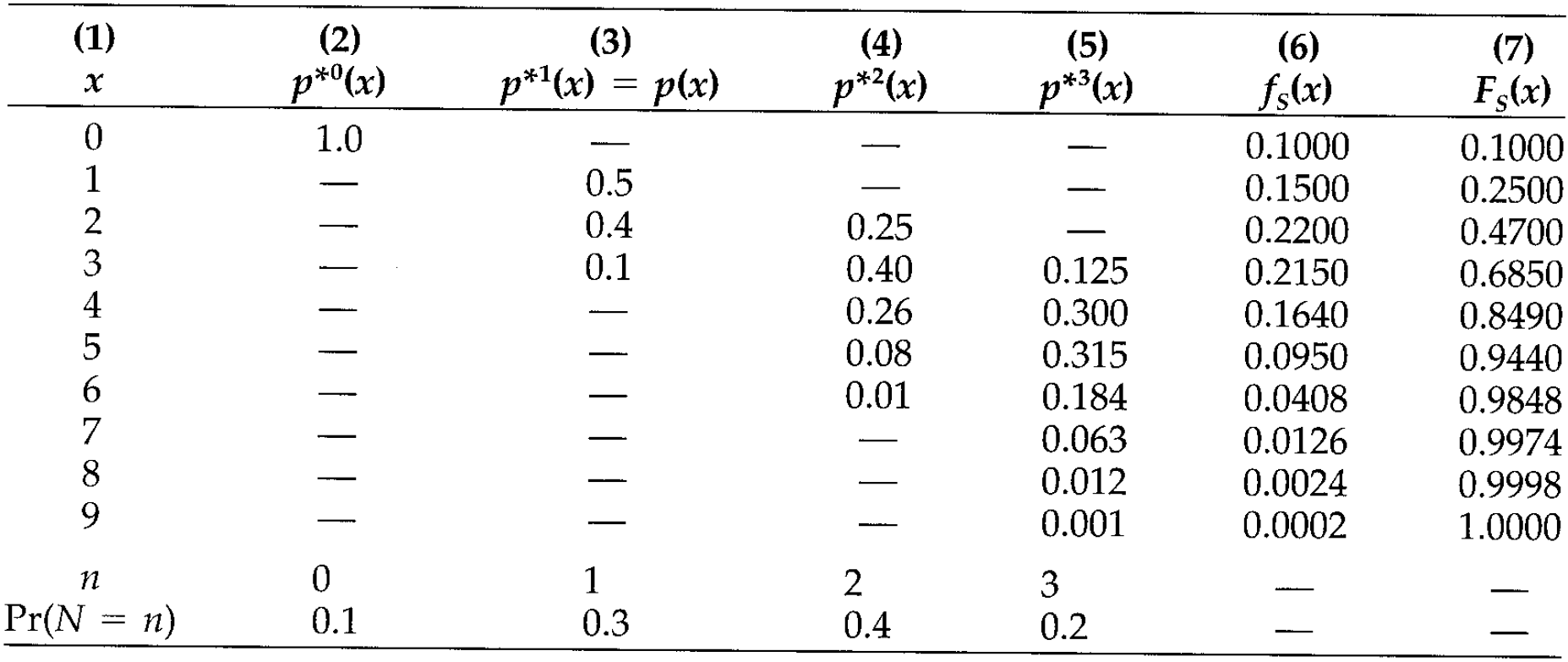
- The convolutions are in done the usual way.
- The number of columns depends on the range of
\(N\). - The
\(f_S(x)\)are the sumproduct of the row\(x\)and row\(\Pr[N=n]\):
$$f_S(3)=0 \cdot 0.1 + 0.1\cdot0.3 + 0.4 \cdot 0.4 + 0.125 \cdot 0.2.$$
Using R #
We will make extensive use of the function aggregateDist from the package actuar (Dutang, Goulet, and Pigeon 2008):
- This function allows for several different aggregate distribution approaches, which will be introduced here (and in Module 4 as the associated theory is presented).
- Here, we show how the function can be used to implement formulas (1) and (2) (using the function
convolvein the background). This corresponds to themethod="convolution"approach.
actuar::aggregateDist(method="convolution"):
- A discrete distribution for
\(Y\)is required. Note that discretisation methods are discussed in Module 4. This is input as a vector of claim amount probability masses after the argumentmodel.sev=. The first element must be\(\Pr[Y=0]\). - There is no restriction on the shape of the frequency distribution, but it must have a finite range.
This is input as a vector of claim number probability masses after the argument
model.freq=. The first element must be\(\Pr[N=0]\). - The outcome of the function is (1). Additional outputs:
plot: to get a pretty plot of the dfsummary: to get summary statisticsmean: to get the meandiff: to get the pmf
- Additional options are:
x.scale: currency units per unit ofsevin the severity model (this allows calculations on multiples of $1)
# Bowers 12.2.2
fy <- c(0, 0.5, 0.4, 0.1)
fn <- c(0.1, 0.3, 0.4, 0.2)
Fs <- aggregateDist("convolution", model.freq = fn, model.sev = fy)
mean(Fs)
## [1] 2.72
pmf <- c(Fs(0), diff(Fs(0:9)))
cbind(s = c(0:9), fs = pmf, Fs = Fs(0:9))
##       s     fs     Fs
##  [1,] 0 0.1000 0.1000
##  [2,] 1 0.1500 0.2500
##  [3,] 2 0.2200 0.4700
##  [4,] 3 0.2150 0.6850
##  [5,] 4 0.1640 0.8490
##  [6,] 5 0.0950 0.9440
##  [7,] 6 0.0408 0.9848
##  [8,] 7 0.0126 0.9974
##  [9,] 8 0.0024 0.9998
## [10,] 9 0.0002 1.0000
summary(Fs)
## Aggregate Claim Amount Empirical CDF:
## Min. 1st Qu. Median Mean 3rd Qu. Max.
## 0.00 2.00 3.00 2.72 4.00 9.00
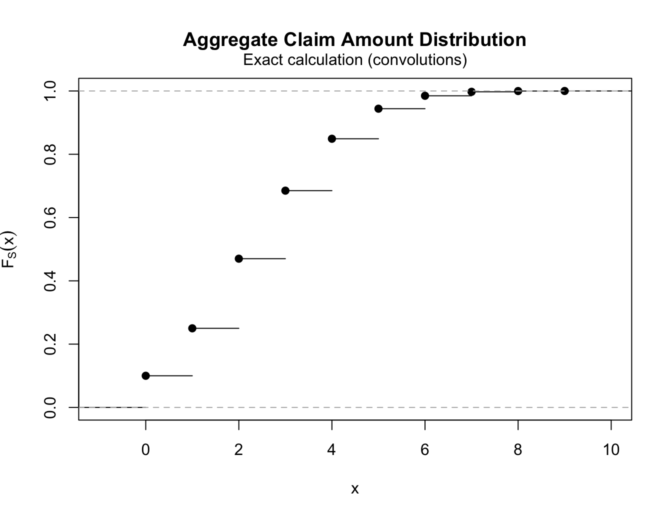
plot(Fs)
Explicit claims count distributions (MW 2.2) #
Introduction #
Exposure #
- It makes no sense to talk about frequency in an insurance portfolio without considering exposure. Chapter 4 of Werner and Modlin (2010) defines exposure as “the basic unit that measures a policy’s exposure to loss”.
- One primary criterion for choosing an exposure base is that it “should be directly proportional to expected loss”. Here we are focussing on frequency, so exposure should be something directly proportional to the expected frequency.
- Wuthrich (2023) calls exposure “volume”, denoted
\(v\), and defines the claims frequency as $$ \frac{N}{v}.$$
Basic models for claims frequency #
- In our case, we will assume that it directly affects the likelihood of a claim to occur - the frequency - such that
\(N/v\)is normalised - MW defines
$$p_k = \Pr[N=k], \quad \text{for }k \in \mathcal{A} \subset \mathbb{N}_0,$$where\(\mathcal{A}\)us the set of possible frequency outcomes. - There are three main assumptions for
\(p_k\):- binomial (with variance less than mean)
- Poisson (with variance equal to the mean)
- negative-binomial (a Poisson with random mean, so that variance is more than the mean)
- A summary table of those distributions is also given in Bowers et al. (1997), see Table 12.3.1 on page 376.
- These all belong to a class of distributions called
\((a,b)\)
Binomial distribution #
- fixed volume
\(v \in \mathbb{N}\) - fixed default probability
\(p \in (0, 1)\)(expected claims frequency) - pmf of
\(N\sim\text{Binom}(v, p)\)is$$p_k =\Pr[N=k]={v \choose k}p^k(1-p)^{v-k}, \quad \text{for all } k \in \{0,\ldots,v\} = \mathcal{A}.$$ - same as a sum of Bernoulli (which is the case
\(v=1\)) - makes sense for homogenous portfolio with unique possible events, such as credit defaults, or deaths in a life insurance model
- In R:
dbinom,pbinom,qbinom,rbinom, wheresizeis\(v\), and whereprobis\(p\) - Note that
\({\binom v k}\)can be computed with the R functionchoose.
Compound binomial model #
The total claim amount \(S\) has a compound binomial distribution
$$S \sim \text{CompBinom}(v,p,G)$$
if \(S\) has a compound distribution with \(N \sim \text{Binom}(v,p)\) for given \(v\in \mathbb{N}\) and \(p\in (0,1)\) and individual claim size distribution \(G\).
Corollary 2.7: Assume \(S_1,\ldots,S_n\) are independent with \(S_j \sim \text{CompBinom}(v_j,p,G)\) for all \(j=1,\ldots,n\). The aggregated claim has a compound binomial distribution with
$$S=\sum_{j=1}^n S_j \sim \text{CompBinom}\left( \sum_{j=1}^n v_j, p,G \right).$$
Exercise NLI3 considers the decomposition of \(S\) into small and large
claims. It shows that \(S_{\text{lc}}\)—the sum of those claims exceeding a
certain threshold \(M\) only (see notation in Example 2.16 later in those slides)—is compound binomial again.
Poisson distribution #
-
fixed volume
\(v > 0\) -
expected claims frequency
\(\lambda >0\) -
pmf of
\(N\sim\text{Poi}(\lambda v)\)is$$p_k =\Pr[N=k]=e^{-\lambda v}\frac{(\lambda v)^k}{k!}\quad \text{for all }k\in \mathcal{A}=\mathbb{N}_0.$$ -
Lemma 2.9: increase volume while keeping
\(E[N]\)fixed in a binomial model leads to a Poisson distribution (more so for small\(p\)compared to\(v\)). -
In R:
dpois,ppois,qpois,rpois, wherelambdais\(\lambda v\)
Compound Poisson model #
The total claim amount \(S\) has a compound Poisson distribution
$$S \sim \text{CompPoi}(\lambda v,G)$$
if \(S\) has a compound distribution with \(N \sim \text{Poi}(\lambda v)\) for given \(\lambda,v>0\) and individual claim size distribution \(G\).
- The compound Poisson distribution has nice properties such as:
- The aggregation property
\(\uparrow\) - The disjoint decomposition property
\(\downarrow\)
- The aggregation property
- These are reviewed in the next section, along with related new techniques for computing the distribution of
\(S\).
Mixed Poisson distribution #
Inhomogeneous portfolio #
- So far we have seen distributions with variance less (binomial) or exactly equal (Poisson) to the mean.
- In reality, actuarial data is often overdispersed, that is, variance is larger than mean.
- This could be due to frequency or severity, but it makes sense that some of this extra variability would come from frequency.
- If we believe in a Poisson frequency for known frequency parameter, then additional uncertainty such as heterogeneity of risks in a portfolio, uncertain conditions (weather, for instance) could be modelled with a random Poisson parameter, and could explain the extra variability.
- This is the idea of a mixed Poisson.
The mixed Poisson distribution #
- Assume random
\(\Lambda \sim H\)with\(H(0)=0\),\(E[\Lambda]=\lambda\), and\(Var(\Lambda)>0\). - Conditionally, given
\(\Lambda\),\(N\sim \text{Poi}(\Lambda v)\)for fixed volume\(v>0\).
We have then
$$\begin{array}{rcl} \displaystyle \Pr[N=n]&=&\int_0^\infty \Pr[N=n|\Lambda=\lambda] d H(\lambda)=\int_0^\infty \frac{e^{-\lambda v}(\lambda v)^n}{n!} d H(\lambda); \\ \\ E[N] &=& E\left[E[N|\Lambda]\right] = E[\Lambda]v=\lambda v; \\ \\ Var(N) &=& E\left[Var(N|\Lambda)\right] + Var\left(E[N|\Lambda]\right)= \lambda v+v^2 Var(\Lambda) > \lambda v; \\ \\ M_N(t) &=&E\left[e^{tN}\right] = E\left[E\left[e^{tN}|\Lambda\right]\right]=E\left[e^{\Lambda v (e^t-1)}\right]=M_\Lambda(v[e^t-1]). \end{array}$$
Example #
If \(\Lambda \sim \text{inverse Gaussian}(\alpha,\beta)\) (Example 12.3.2):
\(N\)is Poisson Inverse Gaussian.- This distribution is the
pigdistribution inactuar, so that you can usedpig,ppig, etc…); see Section 5 of the vignette “distribution” ofactuar. \(\longrightarrow\)\(S\)will be compound inverse Gaussian.
Another example, which is very famous, is \(\Lambda \sim \Gamma\), which leads to the negative-binomial distribution.
Negative-binomial distribution #
Assume \(\lambda\) is the mean, and will be “spread” according to a gamma distribution:
- Define
\(\Lambda = \lambda \Theta\). - Now,
\(\Theta \sim \Gamma(\gamma,\gamma)\)such that $$ E[\Theta]=1 \quad \text{and} \quad Var(\Theta)=\frac{1}{\gamma}$$ and $$ E[\Lambda]=\lambda \quad \text{and} \quad Var(\Lambda)=\frac{\lambda^2}{\gamma}.$$ - If conditionally, given
\(\Theta\),\(N\sim \text{Poi}(\Theta \lambda v)\), then$$N \sim \text{NegBin}(\lambda v, \gamma)$$with volume\(v>0\), expected claims frequency\(\lambda>0\),
and dispersion parameter\(\gamma >0\).
Proof:
$$\begin{array}{rcl} M_N(t) &=& E[e^{tN}]=E\left[ E[e^{tN} | \Theta] \right] = E\left[ e^{\Theta \lambda v (e^t-1)} \right] \\\\ \displaystyle &=& \left( \frac{\gamma}{\gamma-\lambda v (e^t-1)} \right)^\gamma = \left( \frac{\gamma}{\gamma +\lambda v -\lambda v e^t} \right)^\gamma = \left( \frac{\frac{\gamma}{\lambda v +\gamma}}{1 -\frac{\lambda v}{\lambda v +\gamma} e^t} \right)^\gamma, \end{array}$$
which can be recognised as a negative-binomial with probability of “failure”
$$p = \frac{\lambda v}{\lambda v +\gamma}$$
(if we count failures until the \(\gamma\)-th success) so that
$$p_k =\Pr[N=k]={k+\gamma -1 \choose k}p^k(1-p)^{\gamma}$$
In R, use dnbinom, pnbinom, qnbinom, rnbinom, where size is \(\gamma\) and prob is probability of success \(1-p\) (note volume is hidden in \(p\)
and will affect the scale of the distribution).
Interpretation #
\(\Theta\)reflects the uncertainty about the `true’ parameter of the Poisson distribution.
Alternatively, it describes the distributions of “$\lambda$’s” in the population.- In the end we have
$$\begin{array}{rcl} E[N] &=& \lambda v, \\ Var(N) &=& \lambda v \left(1+\frac{\lambda v}{\gamma}\right) > \lambda v,\\ \text{Vco}\left( \frac{N}{v} \right) &=& \sqrt{(\lambda v)^{-1} + \gamma^{-1}}. \end{array}$$
- This additional uncertainty is not diversifiable
(remains even for large\(v\)):$$\text{Vco}\left( \frac{N}{v} \right) = \sqrt{(\lambda v)^{-1} + \gamma^{-1}} \rightarrow \gamma^{-1/2} > 0\quad \text{ for } v \rightarrow \infty.$$
Compound negative-binomial model #
The total claim amount \(S\) has a compound negative-binomial distribution
$$S \sim \text{CompNB}(\lambda v,\gamma,G)$$
if \(S\) has a compound distribution with \(N \sim \text{NegBin}(\lambda v,\gamma)\) for given \(\lambda,v,\gamma>0\) and individual claim size distribution \(G\).
Additional properties and applications of Poisson frequencies #
Theorem 2.12: Aggregation property \(\uparrow\)
#
Assume \(S_1,\ldots,S_n\) are independent with \(S_j \sim \text{CompPoi}(\lambda_j v_j,G_j)\) for all \(j=1,\ldots,n\). Aggregated claims have a compound Poisson distribution
$$S = \sum_{j=1}^n S_j \sim \text{CompPoi}(\lambda v,G),\text{ with}$$
$$v= \sum_{j=1}^n v_j,\quad \lambda = \sum_{j=1}^n \frac{v_j}{v} \lambda_j,\quad G = \sum_{j=1}^n \frac{\lambda_j v_j}{\lambda v} G_j.$$
So what?
- Independent
\(n\)portfolios of losses can be easily aggregated. - Alternatively (or in addition), total claims paid over
\(n\)years are compound Poisson, even if the severity and frequency of losses vary across years. - “Bottom-up” modelling
- In Bowers et al. (1997), this is Theorem 12.4.1.
Example 12.4.1 of Bowers et al. (1997) #
Suppose that \(N_1, N_2,\cdots, N_m\) are independent random variables. Further, suppose that \(N_i\) follows Poisson($\lambda_i$). Let \(y_1,y_2,\cdots, y_m\) be deterministic numbers. What is the distribution of
$$y_1N_1+\cdots+y_mN_m?$$
Theorem 2.14: Disjoint decomposition property \(\downarrow\)
#
Preliminary 1: Add LoBs in the CompPoi formulation #
Let us introduce Lines of Business (“LoB”) in the notation:
- Let the set
\(\{1,\ldots,m\}\)be a partition of the portfolio, or different lines of business (“LoB” thereafter). For instance, we could have\(j\in\{1,2,3\}\)for car\((j=1)\), building\((j=2)\)and liability\((j=3)\)LoBs. - Let
\(\left(p_j^+\right)_{j=1,\ldots,m}\)be a discrete probability distribution on the finite set of sub-portfolios/LoBs\(\{1,\ldots,m\}\)(thereafter just “LoB”). - We assume
$$ p_j^+ >0 \text{ for all }j,$$
that is, the probability of having claims in any of the
\(m\)LoBs is strictly positive. - We further assume that
\(G_j\)is the claim size distribution of LoB\(j\), with\(G_j(0)=0\).
- Finally, we define the mixture distribution by
$$G(y)= \sum_{j=1}^m p_j^+ G_j(y)\quad \text{ for }y \in \mathbb{R}.$$This is the distribution of a claim, if we don’t know which LoB it comes from. - Note that this matches the formulation in the aggregation property Theorem 2.12 with
$$p_j^+ = \frac{\lambda_j v_j}{\lambda v}.$$ - Now, define a discrete random variable
\(I\)which indicates which sub-portfolio/LoB a randomly selected claim\(Y\)belongs to:$$\Pr [I=j]= p_j^+ \quad \text{ for all }j\in \{1,\ldots,m\}.$$
We are now ready to define the following extended compound Poisson model:
- The total claims
\(S = \sum_{i=1}^N Y_i\)has a compound Poisson distribution as defined earlier. - In addition, we assume that
$$ (Y_i,I_i)_{i\ge 1}$$
are
- mutually i.i.d. and independent of
\(N\), - with
\(Y_i\)having marginal distribution function\(G\)with\(G(0)=0\), and \(I_i\)having marginal distribution function given by\(\Pr [I=j]= p_j^+ \quad \text{ for all }j\in \{1,\ldots,n\}\).
- mutually i.i.d. and independent of
Preliminary 2: Partition #
- The random vector
\((Y_1,I_1)\)takes values in\(\mathbb{R}_+ \times \{1,\ldots,m\}\). - On this set we choose a finite sequence of sets
$$A_1, \ldots, A_n$$such that
$$\begin{array}{rcl} A_k \cap A_l &=& \emptyset \text{ for all }k\neq l\quad \text{(no overlap)}; \\ \cup_{k=1}^n A_k &=& \mathbb{R}_+ \times \{1,\ldots,m\} \quad \text{(all-inclusive)}. \end{array}$$
- Such a sequence is called a “measurable disjoint decomposition” or “partition” of
\(\mathbb{R}_+ \times \{1,\ldots,m\}\). - This partition is called “admissible” for
\((Y_1,I_1)\)if for all\(k=1,\ldots,n\)$$p^{(k)} = \Pr[(Y_1,I_1)\in A_k]>0.$$Note\(\sum_{k=1}^n p^{(k)}=1\)due to the properties of the
partition above (no overlap and all-inclusive)
We have two levels of partition:
- Into LoBs:
- Claims are classified according to a sub-portfolio or LoB
- For instance: domestic motor and commercial motor
- The probability of a claim being in LoB
\(j\)is\(p_j^+\) - The indicator for the claim to be in LoB
\(j\)is\(I_j\)
(with probability\(p_j^+\)of being 1)
- Into a second level:
- Claims are classified according to another set of criteria
- For instance: geographical areas NSW and VIC
- The probability of a claim being in geographical area
\(k\)is\(p(k)\)
Theorem 2.14: Disjoint decomposition \(\downarrow\)
#
Assume \(S\) is “doubly partitioned” as described above:
\(S\)fulfills the extended compound Poisson model assumptions above (Preliminary 1).- We chose an admissible partition
\(A_1, \ldots,A_n\)for\((Y_1,I_1)\)(Preliminary 2).
Then the random variable (sum of claims for partition \(k\)):
$$S_k=\sum_{i=1}^N Y_i 1_{\{(Y_i,I_i)\in A_k\}} \sim \text{CompPoi}(\lambda_k v_k,G_k),$$
for \(k=1,\ldots,n\), with
$$\lambda_k v_k = \lambda v p^{(k)} > 0,\quad G_k(y) = \Pr[Y_1 \le y | (Y_1,I_1) \in A_k].$$
Furthermore, the \(S_k\)’s are independent (over \(k\)).
Thinning of the Poisson process #
- Assume that
\(m=1\)(only one LoB) - The disjoint decomposition theorem implies that $$ Y_i = Y_i 1_{{Y_i\in A_1}} + \ldots + Y_i 1_{{Y_i\in A_n}}.$$
- For for each partition
\(A_k\)(defined on the claims) a natural choice is\(v_k=v\)\(\lambda_k = \lambda p^{(k)}\)
- This means that the volume remains constant in each partition, but the expected claims frequencies
\(\lambda_k\)change proportionally to the probabilities of falling in partition\(A_k\),\(k=1,\ldots,n\). - This is called thinning of the Poisson process.
\(\adv\) Sparse vector algorithm
#
If \(S\sim\text{compound Poisson}(\lambda,g(y_i)=\pi_i)\), \(i=1,\ldots,m\) then
$$S=y_1N_1+\ldots+y_mN_m,$$
where the \(N_i\)’s
- represent the number of claims of amount
\(y_i\); - are mutually independent;
- are Poi
\((\lambda_i=\lambda \pi_i).\)
Proof: see tutorial exercise los18. Note also that this is a special case of Theorem 2.14, and is Theorem 12.4.2 of Bowers et al. (1997).
So what?
- Sparse vector algorithm: allows to develop an alternative method for tabulating the distribution of
\(S\)that is more efficient as\(m\)is small. \(S\)can be used to approximate the Individual Risk Model if\(X=Ib\)(see Module 3).
\(\adv\) The sparse vector algorithm
#
(Bowers et al. 1997, Example 12.4.2) Suppose \(S\) has a compound Poisson distribution with \(\lambda =0.8\) and individual claim amount distribution
| $y_i$ | \(\Pr\left[ Y=y_i\right]\) |
|
|---|---|---|
| 1 | 0.250 | |
| 2 | 0.375 | |
| 3 | 0.375 |
Compute \(f_{S}\left( s\right) =\Pr\left[ S=s\right]\) for \(s=0,1,...,6\).
This can be done in two ways:
- Basic method (seen earlier in the lecture): requires to calculate up to the 6th convolution of
\(Y\). - Sparse vector algorithm: requires no convolution of
\(Y\).
Solution - Basic Method
\(x\) |
\(g^{*0}\left(x \right)\) |
\(g\left( x\right)\) |
\(g^{* 2}\left(x\right)\) |
\(g^{* 3}\left( x\right)\) |
\(g^{* 4}\left( x\right)\) |
\(g^{* 5}\left( x\right)\) |
\(g^{* 6}\left( x\right)\) |
\(f_{S}\left( x\right)\) |
|---|---|---|---|---|---|---|---|---|
| 0 | 1 | - | - | - | - | - | - | 0.4493 |
| 1 | - | 0.250 | - | - | - | - | - | 0.0899 |
| 2 | - | 0.375 | 0.0625 | - | - | - | - | 0.1438 |
| 3 | - | 0.375 | 0.1875 | 0.0156 | - | - | - | 0.1624 |
| 4 | - | - | 0.3281 | 0.0703 | 0.0039 | - | - | 0.0499 |
| 5 | - | - | 0.2813 | 0.1758 | 0.0234 | 0.0010 | - | 0.0474 |
| 6 | - | - | 0.1406 | 0.2637 | 0.0762 | 0.0073 | 0.0002 | 0.0309 |
\(n\) |
0 | 1 | 2 | 3 | 4 | 5 | 6 | |
\(\Pr[N=n]=e^{-0.8}\frac{\left( 0.8\right) ^{n}}{n!}\) |
0.4493 | 0.3595 | 0.1438 | 0.0383 | 0.0077 | 0.0012 | 0.0002 |
- The convolutions are done in the usual way.
- The
\(f_S(x)\)are the sumproduct of the row\(x\)and row\(\Pr[N=n]\). - The number of convolutions (and thus of columns) will increase by 1 for each new value of
\(f_S(x)\), without bound!
Solution - Sparse vector algorithm
Thanks to Theorem 2.12, we can write \(S=N_1+2N_2+3N_3\)
\(x\) |
\(\Pr\left[ N_{1}=x\right]\) |
\(\Pr\left[ 2N_{2}=x\right]\) |
\(\Pr\left[ 3N_{3}=x\right]\) |
\(\Pr\left[ N_{1}+2N_{2}=x\right]\) |
\(f_{S}\left( x\right)\) |
|---|---|---|---|---|---|
| 0 | 0.818731 | 0.740818 | 0.740818 | 0.606531 | 0.449329 |
| 1 | 0.163746 | 0 | 0 | 0.121306 | 0.089866 |
| 2 | 0.016375 | 0.222245 | 0 | 0.194090 | 0.143785 |
| 3 | 0.001092 | 0 | 0.222245 | 0.037201 | 0.162358 |
| 4 | 0.000055 | 0.033337 | 0 | 0.030974 | 0.049906 |
| 5 | 0.000002 | 0 | 0 | 0.005703 | 0.047360 |
| 6 | 0.000000 | 0.003334 | 0.033337 | 0.003288 | 0.030923 |
\(x_i\) |
1 | 2 | 3 | ||
\(\lambda _{i}=\lambda \pi_i\) |
0.2 | 0.3 | 0.3 | ||
\(\Pr[N_i=x/i]\) |
\(e^{-0.2}\frac{\left( 0.2\right) ^{x}}{x!}\) |
\(e^{-0.3}\frac{\left(0.3\right) ^{x/2}}{(x/2)!}\) |
\(e^{-0.3}\frac{\left( 0.3\right) ^{x/3}}{(x/3)!}\) |
The \(f_S(x)\) are convolution, e.g.:
$$(5)[3]=.818731\cdot0+.163746\cdot.222245+.016375\cdot0+.001092\cdot.740818$$
$$(6)[3]=.740818\cdot.037201+0\cdot.194090+0\cdot.121306+.222245\cdot.606531$$
Note that only two convolutions are needed: columns (5) and (6).
Example 2.16: Large claim separation #
- This is a very important (and convenient) application of the Disjoint decomposition property (Theorem 2.14).
- Attritional and catastrophic claims often have very different distributions (different
\(G\)’s); see also https://www.actuaries.digital/2022/01/10/catastrophe-vs-standard-loss-modelling/ - The idea here is to divide the claims into different layers with different distributions:
- Small claims are modelled using a parametric distribution for which it is easy to obtain the distribution of the compound distribution, potentially even approximated with a normal distribution thanks to volume and light right tail;
- Large claims are typically modelled with a Pareto distribution with threshold
\(M\)and tail parameter\(\alpha>1\)(see Module 6 for a justification of this, and for the choice of an appropriate\(M\)). The could also be “modelled” (see article above)
Assuming two layers:
- We choose a large claims threshold
\(M>0\)such that$$0 < G(M) < 1,$$that is, there is probability mass on either size of\(M\). - We define the partition
$$A = A_{\text{sc}} = \{Y_1 \le M\} \quad \text{and} \quad A^c = A_{\text{lc}} = \{Y_1>M\}.$$ - Assume that
$$S \sim \text{CompPoi}(\lambda v, G).$$ - We now define the small and large claims layers as
$$\begin{array}{rcl} S_{\text{sc}} &=& \sum_{i=1}^N Y_i 1_{\{Y_i\le M\}}, \text{ and}\\ S_{\text{lc}} &=& \sum_{i=1}^N Y_i 1_{\{Y_i > M\}}, \end{array}$$respectively.
- Theorem 2.14 implies that
\(S_{\text{sc}}\)and\(S_{\text{lc}}\)are and compound Poisson distributed with$$\begin{array}{rcl} S_{\text{sc}} &\sim & \text{CompPoi}(\lambda_{\text{sc}}v = \lambda G(M)v, \\ &&\quad\quad\quad\quad G_{\text{sc}}(y)=\Pr[Y_1\le y|Y_1\le M]), \text{ and} \\ S_{\text{lc}} &\sim & \text{CompPoi}(\lambda_{\text{lc}}v = \lambda (1-G(M))v, \\ &&\quad\quad\quad\quad G_{\text{lc}}(y)=\Pr[Y_1\le y|Y_1> M]), \end{array}$$respectively. - The distribution of
$$S=S_{\text{sc}} + S_{\text{lc}}$$can then be obtained by a simple convolution of distributions of\(S_{\text{sc}}\)and\(S_{\text{lc}}\)(thanks to independence); see Module 4 for examples ().
\(\adv\) Parameter estimation (MW 2.3)
#
\(\adv\) Introduction
#
\(\adv\) Estimation methods
#
You should be familiar with the main estimation methods:
- Method of moments
- Maximum likelihood estimation
Here the problem is slightly complicated because our observations may not be directly comparable due to varying exposures \(v\)’s.
Assume that \((N_1,\ldots,N_T)'\) is the vector of observations.
\(\adv\) What to do with volumes? Lemma 2.26
#
- The key idea here is to find the minimum variance method of moments estimator, when the volumes across the observations can vary.
- This is what is different from a straight method of moments estimator, and explains why we need to think it through: how to deal with those volumes?
- Assume there exist strictly positive volumes
\(v_1,\ldots, v_T\)such that the components of\((N_1/v_1,\ldots,N_T/v_T)\)are independent with$$\lambda = E\left[\frac{N_t}{v_t}\right]\text{ and } \tau_t^2 = Var\left(\frac{N_t}{v_t}\right) \in (0,\infty),$$for all\(t = 1,\ldots,T\).
Lemma 2.26 states that the unbiased, linear estimator for \(\lambda\) with minimal variance is given by
$$\widehat{\lambda}^{\text{MV}}_T = \left( \sum_{t=1}^T \frac{1}{\tau_t^2}\right)^{-1} \sum_{t=1}^T \frac{N_t/v_t}{\tau_t^2},$$
with variance
$$Var(\widehat{\lambda}^{\text{MV}}_T) = \left( \sum_{t=1}^T \frac{1}{\tau_t^2} \right)^{-1}.$$
Note:
- We haven’t made any distributional
assumption yet - this estimates
\(E\left[\frac{N_t}{v_t}\right]\)via method of moments, taking the\(v_t\)’s into account in an optimal way (in the sense that it minimises the variance of the estimator). - The superscript “MV” stands for “minimal variance”.
\(\adv\) Method of moments
#
\(\adv\) Binomial and Poisson cases
#
Unbiased, minimal variance estimators:
- binomial case for
\(p\):$$\widehat{p}_T^{\text{MV}} = \frac{1}{\sum_{s=1}^T v_s} \sum_{t=1}^T N_t = \sum_{t=1}^T \frac{v_t}{\sum_{s=1}^T v_s} \frac{N_t}{v_t} \sim$$Furthermore,\(\sum_{t=1}^T N_t\sim\text{Binom}(\sum_{s=1}^T v_s,p)\), which means we know the distribution of\(\widehat{p}_T^{\text{MV}}\). - Poisson case for
\(\lambda\):$$\widehat{\lambda}_T^{\text{MV}} = \frac{1}{\sum_{s=1}^T v_s} \sum_{t=1}^T N_t = \sum_{t=1}^T \frac{v_t}{\sum_{s=1}^T v_s} \frac{N_t}{v_t}$$Here,\(\sum_{t=1}^T N_t\sim\text{Poi}(\lambda \sum_{s=1}^T v_s)\).
\(\adv\) Negative binomial case
#
More complicated, because:
$$E\left[\frac{N_t}{v_t}\right] = \lambda \text{ and } Var\left(\frac{N_t}{v_t}\right) = \lambda/v_t + \lambda^2/\gamma= \tau_t^2,$$
Unbiased (but not guaranteed minimal variance):
$$\widehat{\lambda}^{\text{NB}}_T = \frac{1}{\sum_{s=1}^T v_s} \sum_{t=1}^T N_t = \sum_{t=1}^T \frac{v_t}{\sum_{s=1}^T v_s} \frac{N_t}{ v_t}$$
\(\adv\) We need a sense of the dispersion for estimating the dispersion parameter \(\gamma\).
Let the weighted sample variance
$$\widehat{V}_T^2 = \frac{1}{T-1} \sum_{t=1}^T v_t \left( \frac{N_t}{v_t} - \widehat{\lambda}^{\text{NB}}_T \right) ^2.$$
Then we have
$$\widehat{\gamma}^{\text{NB}}_T = \frac{(\widehat{\lambda}^{\text{NB}}_T)^2}{\widehat{V}_T^2 -\widehat{\lambda}^{\text{NB}}_T}\frac{1}{T-1} \left( \sum_{t=1}^T v_t - \frac{ \sum_{t=1}^T v_t^2}{ \sum_{t=1}^T v_t} \right),$$
ONLY if \(\widehat{V}_T^2 >\widehat{\lambda}^{\text{NB}}_T\). Otherwise use Poisson or binomial.
\(\adv\) Maximum likelihood estimators
#
\(\adv\) Binomial and Poisson cases
#
Estimators are identical to method of moments estimators. Or conversely, the MLE estimators are actually unbiased.
- binomial case for
\(p\):$$\widehat{p}_T^{\text{MLE}} = \frac{1}{\sum_{s=1}^T v_s} \sum_{t=1}^T N_t = \sum_{t=1}^T \frac{v_t}{\sum_{s=1}^T v_s} \frac{N_t}{v_t}=\widehat{p}_T^{\text{MV}}$$ - Poisson case for
\(\lambda\):$$\widehat{\lambda}_T^{\text{MLE}} = \frac{1}{\sum_{s=1}^T v_s} \sum_{t=1}^T N_t = \sum_{t=1}^T \frac{v_t}{\sum_{s=1}^T v_s} \frac{N_t}{v_t}= \widehat{\lambda}_T^{\text{MV}}$$
\(\adv\) Negative binomial case
#
Assume \(N_1,\ldots, N_T\) are independent and \(\text{NegBin}(\lambda v_t,\gamma)\). The MLE \((\widehat{\lambda}_T^{\text{MLE}},\widehat{\gamma}^{\text{MLE}}_T)\) are the solution of
$$\frac{\partial}{\partial (\lambda, \gamma)} \sum_{t=1}^T \log {N_t +\gamma -1 \choose N_t} + \gamma \log (1-p_t) + N_t \log p_t = 0,$$
with \(p_t = \lambda v_t / (\gamma + \lambda v_t) \in (0,1)\).
The \((a,b,0)\) and \((a,b,1)\) classes of distributions
#
The \((a,b)\) class of Panjer distributions (4.2.1)
#
A class of distributions has the following property
$$ \Pr[N=n]=\left(a+\frac{b}{n}\right)\Pr[N=n-1], \text{ or } \frac{p_k}{p_{k-1}}=\left(a+\frac{b}{k}\right). $$
This is the \((a,b)\) class of “Panjer distributions”. This means that \(\Pr[N=n]\) can be obtained recursively with initial value \(\Pr[N=0]\); see Wuthrich (2023), Definition 4.6.
The exhaustive list of its members (see Wuthrich 2023 Lemma 4.7) is
| Distribution | \(a\) |
\(b\) |
\(\Pr[N=0]\) |
|---|---|---|---|
Poisson \(\left( \lambda \right)\) |
\(0\) |
\(\lambda\) |
\(e^{-\lambda}\) |
Neg Bin \(\left( \gamma,p\right)\) |
\(p\) |
\((\gamma-1)p\) |
\((1-p)^\gamma\) |
Binomial \(\left( m,p\right)\) |
\(-p/(1-p)\) |
\((m+1)p/(1-p)\) |
\((1-p)^m\) |
Exercise: prove the results in the above table!
(Note the Negative Binomial is parametrised as per Proposition 2.20 in Wuthrich (2023) (second definition))
First three cumulants of the \((a,b)\) family
#
| Distribution | \(E[N]\) |
\(Var(N)\) |
\(E\left[(N-E[N])^3\right]\) |
|---|---|---|---|
Poisson \(\left( \lambda \right)\) |
\(\lambda\) |
\(\lambda\) |
\(\lambda\) |
Neg Bin \(\left( \gamma,p\right)\) |
\(\displaystyle\frac{\gamma p}{1-p}\) |
\(\displaystyle \frac{\gamma p}{(1-p)^2}\) |
\(\displaystyle \frac{\gamma p(1+p)}{(1-p)^3}\) |
Binomial \(\left( m,p\right)\) |
\(mp\) |
\(mpq\) |
\(mpq(q-p)\) |
Exercise:
- check these results using the cgf
- find the first 3 cumulants of
\(S\), as well as\(\varsigma_S\)for each member of the family
\(\adv\) actuar and the \((a,b,1)\) class
#
- The package
actuarextends the definition above to allow for zero-truncated and zero-modified distributions. - The Poisson, binomial and negative-binomial (and special case geometric) are all well supported in Base R with the
d,p,qandrfunctions. - If one takes the Panjer equation for granted, then we can think of
\(p_0\)as the mass that will make the pmf add up to one:$$\text{given Panjer}: p_0 \text{ is such that } \sum_{k=0}^\infty p_k = 1.$$ - We introduce here the
\((a,b,1)\)class which extends the idea above so that we have more freedom on the mass at 0. - The reference for this section is Section 4 of the
vignette “distribution” of
actuar
\(\adv\) The \((a,b,1)\) class of distributions
#
A discrete random variable is a member of the ** \((a,b,1)\) class of distributions** if there exist constants \(a\) and \(b\) such that
$$\frac{p_k}{p_{k-1}}=a+\frac{b}{k},\quad **k=2,3,\ldots**.$$
Note:
- The recursion starts at
\(k=2\)for the\((a,b,1)\)class. - The extra freedom allows the probability at zero to be set to any arbitrary number
\(0\le p_0 \le 1\)
\(\adv\) Zero-truncated distributions
#
- Setting
\(p_0=0\)in the\((a,b,1)\)class defines the subclass of zero-truncated distributions - Members are the zero-truncated Poisson (
actuar::ztpois), zero-truncated binomial (actuar::ztbinom), zero-truncated negative-binomial (actuar::ztnbinom), and the zero-truncated geometric (actuar::ztgeom). - Let
\(p_k^T\)denote the probability mass at\(k\)for a zero-truncated distribution (“$T$” for truncated). We have$$p_k^T = \left\{ \begin{array}{ll} 0, & k=0; \\ \frac{p_k}{1-p_0}, & k=1,2,\ldots. \end{array}\right.,$$where\(p_k\)is the probability mass of the corresponding member of the\((a,b,0)\)— that is,\((a,b)\)— class. actuarprovides thed,p,q, andrfunctions of the zero-truncated distributions mentioned above.
\(\adv\) Zero-modified distributions
#
- Setting
\(p_0\equiv p_0^M\)\((0<p_0^M<1)\)in the\((a,b,1)\)class defines the subclass of zero-modified distributions (“$M$” for “modified”) - These distributions are discrete mixtures between a degenerate distribution at zero, and the corresponding distribution from the
\((a,b,0)\)class. - Let
\(p_k^M\)denote the probability mass at\(k\)for a zero-modified distribution. We have then$$p_k^M = \left( 1-\frac{1-p_0^M}{1-p_0}\right)1_{\{k=0\}} + \frac{1-p_0^M}{1-p_0}p_k.$$Alternatively,$$p_k^M = \left\{ \begin{array}{ll} p_0^M, & k=0; \\ \frac{1-p_0^M}{1-p_0}p_k, & k=1,2,\ldots. \end{array}\right.,$$where\(p_k\)is the probability mass of the corresponding member of the\((a,b,0)\)class.
- Quite obviously, zero-truncated distributions are zero-modified distributions with
\(p_0^M=0\), and$$p_k^M = p_0^M 1_{\{k=0\}}+(1-p_0^M)p_k^T.$$ - Members are the zero-modified Poisson (
actuar::zmpois), zero-modified binomial (actuar::zmbinom), zero-modified negative-binomial (actuar::zmnbinom), and the zero-modified geometric (actuar::zmgeom).actuarprovides thed,p,q, andrfunctions of the zero-truncated distributions mentioned above.
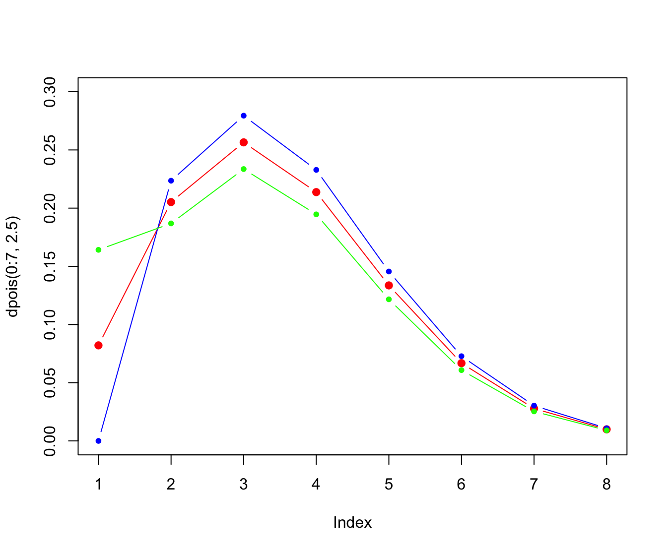
plot(dpois(0:7, 2.5), pch = 20, col = "red", ylim = c(0, 0.3),
  cex = 1.5, type = "b")
points(dztpois(0:7, 2.5), pch = 20, col = "blue", type = "b")
points(dzmpois(0:7, 2.5, 2 * dpois(0, 2.5)), pch = 20, col = "green",
  type = "b")
References #
Bowers, Newton L. Jr, Hans U. Gerber, James C. Hickman, Donald A. Jones, and Cecil J. Nesbitt. 1997. Actuarial Mathematics. Second. Schaumburg, Illinois: The Society of Actuaries.
Dutang, Christophe, Vincent Goulet, and Mathieu Pigeon. 2008. “Actuar: An r Package for Actuarial Science.” Journal of Statistical Software 25 (7).
Werner, Geoff, and Claudine Modlin. 2010. Basic Ratemaking. Casualty Actuarial Society.
Wuthrich, Mario V. 2023. “Non-Life Insurance: Mathematics & Statistics.” Lecture notes. RiskLab, ETH Zurich; Swiss Finance Institute.